Advisor's Opinion on Situation Report No. 6, 2016

OPINION ON SITUATION REPORT NO. 6[1]

1. Recommendation

The period since the presentation of Situation Report No. 5 was marked by mildly unfavorable news from the real economy: lower-than-forecast growth in wages, household consumption, and fixed investment in the second quarter, and weak July figures for retail sales, foreign trade, and industrial production. GDP growth itself was higher than forecast, but only because of lower import growth and a smaller decline in inventories. The true momentum of the economy in the second quarter is probably understated by the method of adjusting for the number of calendar days, while the July data are dragged down by plant-wide holidays. What I consider important is that the inflation forecast has repeatedly been fulfilled. Moreover, the ECB is not yet discussing an extension of its asset purchase program. Like Situation Report No. 6, then, I assess the risks to the August forecast as balanced, and I believe the conditions relevant for the timing of the exit have not changed. I therefore recommend leaving the settings of interest rates and the parameters of the exchange rate commitment unchanged. In this opinion I show in three ways that the available information on the effects of quantitative easing and from the derivatives market points to a milder appreciation of the koruna after the exit than the forecast assumes, even after the effects of this month's speculation are taken into account.

The first line of argument is based on a comparison of shadow monetary policy rates for the ECB and the CNB. The interest rate differential that emerges from this analysis has the opposite sign to the one the forecast works with: the CNB shadow rate is more negative than the ECB shadow rate. The second compares interest rates that can actually be traded and uses the implied koruna yield derived from the forward exchange rate. The resulting interest rate differential is negligible and, for most of this year, negative, just as in the first case. In the third part of the analysis I discuss the forward curve and present empirical support for the stylized fact that markets take seriously the "hard" commitment (that is, not abandoning the use of the exchange rate as a monetary policy instrument before the end of this year) rather than the "soft" one (that is, the probabilistic formulation of an exit in mid-2017). Forward exchange rates are consistent with the expectation that within two years the koruna will not appreciate beyond roughly 26.60 CZK/EUR. This expectation does not reflect possible short-term volatility of the exchange rate, within which the koruna could temporarily appreciate further just after the exit, but which will have no consequences for price stability.

These considerations imply that under current circumstances it is not appropriate to extend the hard commitment and that a one-off exit without backstops will be relatively easy to carry out. Since the koruna should appreciate less after the exit than the forecast assumes, one can imagine an exit earlier than in the middle of next year. Pushing the hard commitment back would narrow the room for maneuver of monetary policy in the first half of 2017, but it would provide free hedging to exporters and temporarily damp speculation. I do not find either of these arguments for shifting the commitment convincing, however. First, the price of one-year hedging averaged CZK 0.15 per euro in the summer and thus did not represent a significant cost. Second, speculative attacks do enlarge the CNB balance sheet, and thus mean higher accounting losses in the future, but that is a smaller risk to meeting the inflation target than a significant potential for koruna appreciation after the exit (other things equal, the increase in koruna liquidity supplied while the commitment lasts leads to a smaller future potential for the koruna to appreciate).

It also follows that in the current situation I consider it inappropriate to introduce statutory negative rates, which would limit speculation, but in doing so would merely push the problem of koruna appreciation into the post-exit period, in connection with rate normalization. Important segments of the financial market already operate de facto under (often quite deeply) negative interest rates, a consequence of the combination of the ECB's negative rates and quantitative easing with the CNB's exchange rate commitment. Statutory negative rates on the order of a few tens of basis points would therefore not solve much. Over the long run, though, I am not so optimistic, and I fear that negative rates will be hard to avoid.[2] Neutral interest rates have been falling worldwide over the past two decades, and in the euro area they are already negative (Holston et al., 2016). Under such conditions we will run into the zero lower bound in most recessions. However effective the exchange rate commitment is, it is not fully flexible, and it is a question whether it will be appropriate to resort to it repeatedly. An interesting aspect of the current situation is that we can watch negative rates working in practice in the Czech Republic, including a number of their side effects. In the coming years the share of cashless transactions should also rise faster, as contactless payment cards and other innovations are used more and more.

2. Shadow rates

The g3 model uses shadow Euribor rates to capture the effects of unconventional monetary policy in the euro area. I see a certain inconsistency in the fact that in the uncovered interest parity condition these shadow rates are compared with official (non-shadow) PRIBOR rates, even though supplying koruna liquidity under the CNB's exchange rate commitment is also a form of quantitative easing, so the "reference" PRIBOR rates do not reflect the true degree of monetary policy easing. On top of that, the current ECB shadow rate is constructed by extrapolation from the NiGEM model, which relies on estimates of the effects of unconventional policies on GDP, estimates that are themselves subject to uncertainty. Around the world, shadow rates built from the yield curve are used much more often,[3] and I present estimates of them for the Czech Republic in this opinion.

The best-known method for computing shadow rates is presented in Wu and Xia (2016), but it turns out that it cannot currently be used in the Czech setting (some of the data needed for a credible calculation are not available).[4] Shadow rates for the Czech Republic can, however, be computed relatively easily using the second best-known approach, introduced in Krippner (2015). That author also shows that his method is usually more robust than the Wu and Xia approach, so changes in the model specification do not affect the results as strongly. The principle of the estimation is as follows: from the historical shape of the government bond yield curve, its short end is computed for a situation in which no lower bound on rates existed. A shadow monetary policy rate constructed in this way reflects the influence that monetary policy has on interest rates at longer maturities (overall monetary conditions including the effects of expectations, forward guidance, and so on).

For the calculation I use data constructed within the project of Dvorak et al. (2016), which are based on figures from the MtS system (and BCPP) and which show a lower error rate, that is, fewer data points with unrealistic prices, than Bloomberg or Reuters Datastream. Besides, using the zero-coupon curve straight from Bloomberg/Datastream runs into 1) missing values for some of the needed maturities, 2) time series that are too short, especially at longer maturities, and 3) insufficient transparency about the methodology used in constructing the curves, which can have a non-negligible effect on the resulting values. The model for computing the shadow rate in this opinion uses the dynamic two-factor specification of Nelson and Siegel (1987) and is estimated with an iterated extended Kalman filter.

Chart 1: The CNB shadow rate

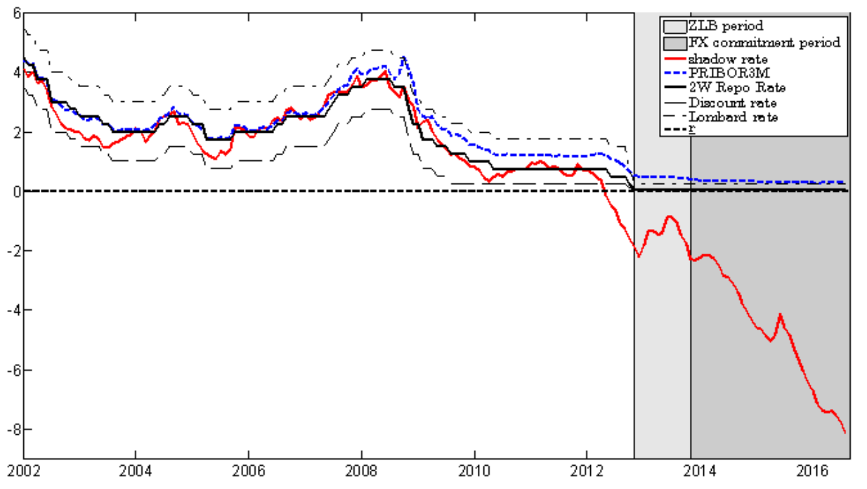
Chart 1 shows that until 2012 the estimated shadow rate tracks the main monetary policy rate fairly well (the undershooting episode in 2002 may be related to the interventions of that time). The three-month PRIBOR roughly matches both the shadow and the non-shadow repo rate until 2008; since then it has been well above them, and from 2012 on it stops being informative in any way about the degree of monetary policy easing as measured by the shadow rate. The shadow rate itself dips into negative territory as early as 2012, perhaps in connection with the formation of expectations of further easing and with spillovers from ECB monetary policy, which gradually pushed down the yields on Czech government bonds. The shadow rate stays mildly negative until the launch of the exchange rate commitment, after which it falls sharply, reaching −8% by September 2016.

Such a deeply negative value looks surprising, especially compared with the only mildly negative ECB shadow rate computed from NiGEM and currently used in the forecast; but the ECB shadow rate presented by Krippner himself (Chart 2) is at present similarly deeply negative, only slightly higher (still below −7%). The Wu and Xia (2016) estimates for the ECB are now also very deeply negative. Chart 2 shows clearly the influence of expectations on the shadow rate: in the second quarter of last year, bond yields in euro area countries rose temporarily but significantly in response to a series of optimistic reports on inflation and from the real economy, which reduced expectations of further monetary policy easing by the ECB. This showed up as a temporary increase in the shadow rate as a measure of the overall ease of monetary policy, which, absent the effective lower bound, would be reflected in the main monetary policy rate.

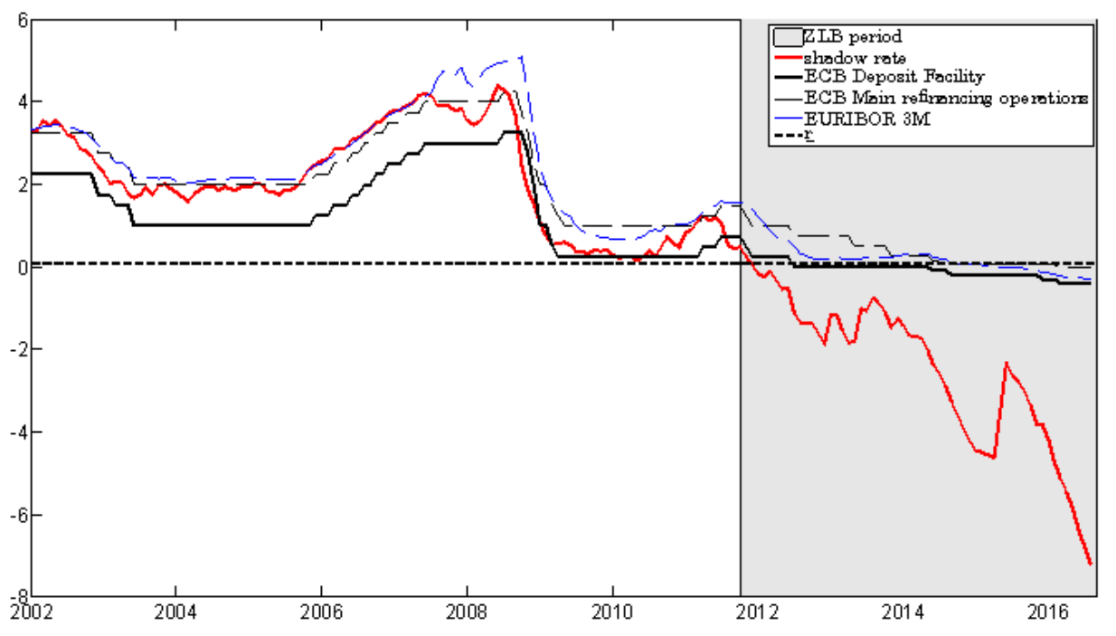
Chart 2: The ECB shadow rate (calculated by L. Krippner, RBNZ)

Overall, the analysis in this section indicates that the interest rate differential measured by shadow rates has the opposite sign to the one assumed by the g3 model: the shadow rate is more negative for the CNB than for the ECB.[5] This reflects the fact that maintaining the exchange rate commitment matches any easing of monetary policy by the ECB (which in effect reflects the monetary trilemma), while the very establishment of the commitment, and possibly also the additional euro purchases in response to speculative attacks, ease domestic monetary policy beyond the easing delivered by the ECB, mainly by pushing down bond yields and other interest rates. The CNB shadow rate has been below the ECB shadow rate precisely since last summer, when the first such speculation occurred.

3. The interest rate differential

However useful shadow rates may be as an analytical tool in certain situations, they are an academic construct, not actual interest rates at which market participants could trade. The question thus arises whether the interest parity condition should not compare interest rates that can actually be traded. For the ECB one can simply use the three-month (non-shadow) Euribor, because the interbank market based on it still functions in the euro area after a fashion, but a problem arises with Czech rates, since PRIBOR is a de facto dead rate. The effective yield on the marginal koruna invested from abroad is even lower than the CNB's deposit/repo rate, for four reasons: 1) market participants perceive some risk that the CNB will introduce statutory negative rates and try to avoid longer-term deposits in accounts, 2) regulation leads to counterparty limits, and for many investors it is safer to buy an asset, typically a government bond or a Treasury bill, instead of depositing in an account, 3) domestic banks are not keen to accept further liquidity because it inflates their balance sheets, which worsens indicators like ROA, 4) for many investors and speculators it is complicated to manage koruna liquidity, so they use currency derivatives in which the funds are converted into euros or dollars for a time. Because forward exchange rates, thanks to the existence of the exchange rate commitment, are typically not weaker than 27 CZK/EUR, the implied koruna yield on such an operation is negative.

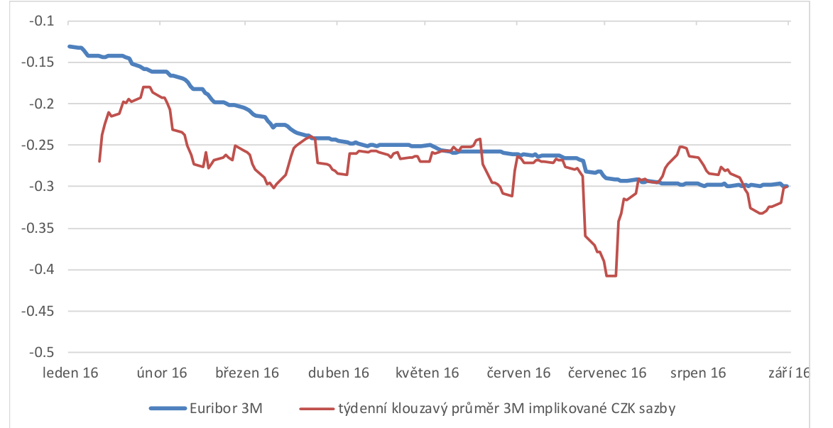
Chart 3: The three-month Euribor and the implied koruna rate

−0.5 January 16 February 16 March 16 Euribor 3M April 16 May 16 June 16 July 16 August 16 weekly moving average of the 3M implied CZK rate September 16

Chart 3 shows that there is no large differential between Euribor and the implied koruna rate (here I use a weekly moving average because the forward exchange rate, and hence the implied rate derived from it, is quite volatile). For most of this year, the implied three-month koruna yield has actually been more negative than the three-month Euribor. The negative implied yield then spills over into other areas of the financial market, where we observe, for example, markedly negative interest rates on government bonds. Anecdotal evidence also suggests that although the three-month bid prices quoted on Bloomberg are positive, when one bank actually wants to deposit money with another, the rate actually offered tends to be negative (easily around −0.3%). So this view, too, does not suggest that any significant positive differential between koruna and euro rates really exists. A simple comparison of the yields on Czech and, say, Austrian government bonds leads to a similar conclusion, and the differential assumed by the forecast, effectively plus 1.8 percentage points (non-shadow PRIBOR vs. shadow Euribor according to NiGEM), is thus in my view overstated by an order of magnitude.

4. Forward exchange rates

The so-called unbiasedness hypothesis holds that the best estimate of the future spot exchange rate is the current forward rate (Fama, 1984). The empirical evidence for this hypothesis is mixed, but forwards are backed by real trades, so I tend to trust them more than the estimates of analysts who put none of their own money into the prediction (various estimates of the "fair exchange rate" ranging between 22 and 26). In theory, the price of a forward should also reflect the effect of a missing counterparty, which may help explain why the forward is weaker than the exchange rate in the forecast. If the market on average believes the koruna will appreciate to 26 CZK/EUR within two years, the two-year forward should trade near that level. If, despite that expectation, the forward cost, say, 26.60, a trader in the forward market would buy the koruna and realize a solid profit. The whole forward curve then gives us interesting information about market expectations for the path of the koruna in the months and years ahead. In this section I use bid prices, that is, the cost of a forward purchase of korunas.

27.04 27.02 27 26.98 26.96 26.94 26.92 26.9 26.88 26.86 26.84 26.82 September 16

Chart 4: The CZK/EUR forward curve

the "hard" commitment

the "soft" commitment January 17 April 17 July 17 October 17 February 18 May 18 August 18

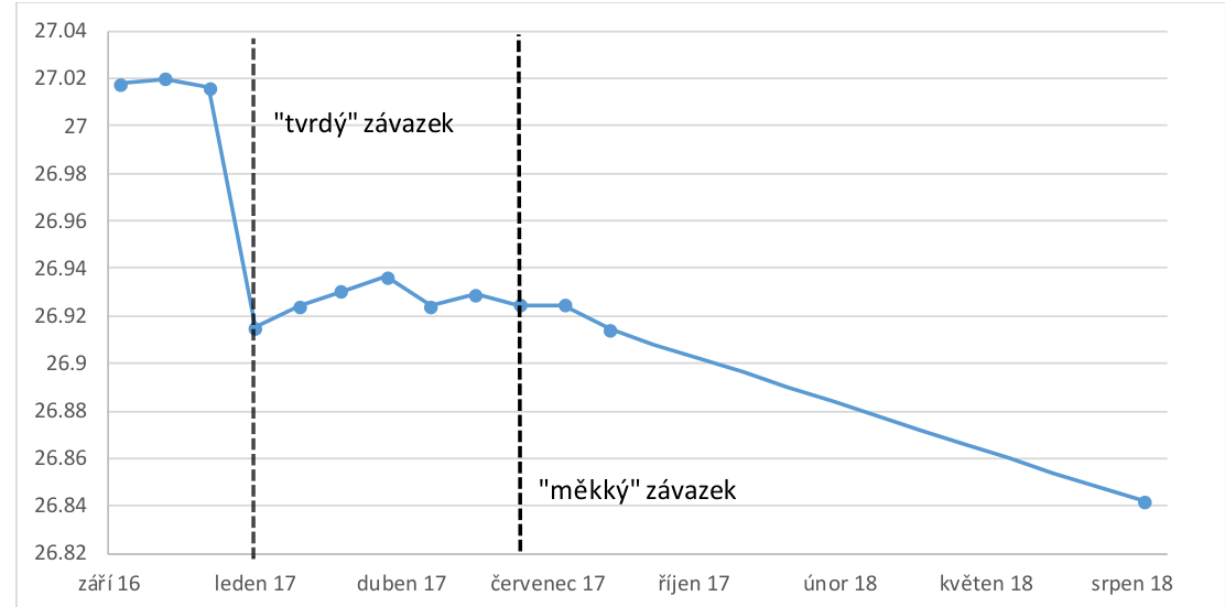
Chart 4 shows that the market expects some appreciation after the expiry of the "hard" commitment (that is, at the beginning of January 2017), but expects no reaction to the expiry of the "soft" commitment (mid-2017). Given the wording of the commitment (end of the year, middle of the year), it makes most sense to examine the forward curve from the beginning of a month, so that a forward several months out also refers to the beginning of a month, the earliest point at which the commitment can be exited; the chart refers to the beginning of September. The forward curve has had this shape for most of this year, though: a curve from the beginning of June, for example, would show the same picture, appreciation in January 2017 and no jump in mid-2017. So this is nothing new that first appeared in September.[6]

Chart 5: The two-year CZK/EUR forward

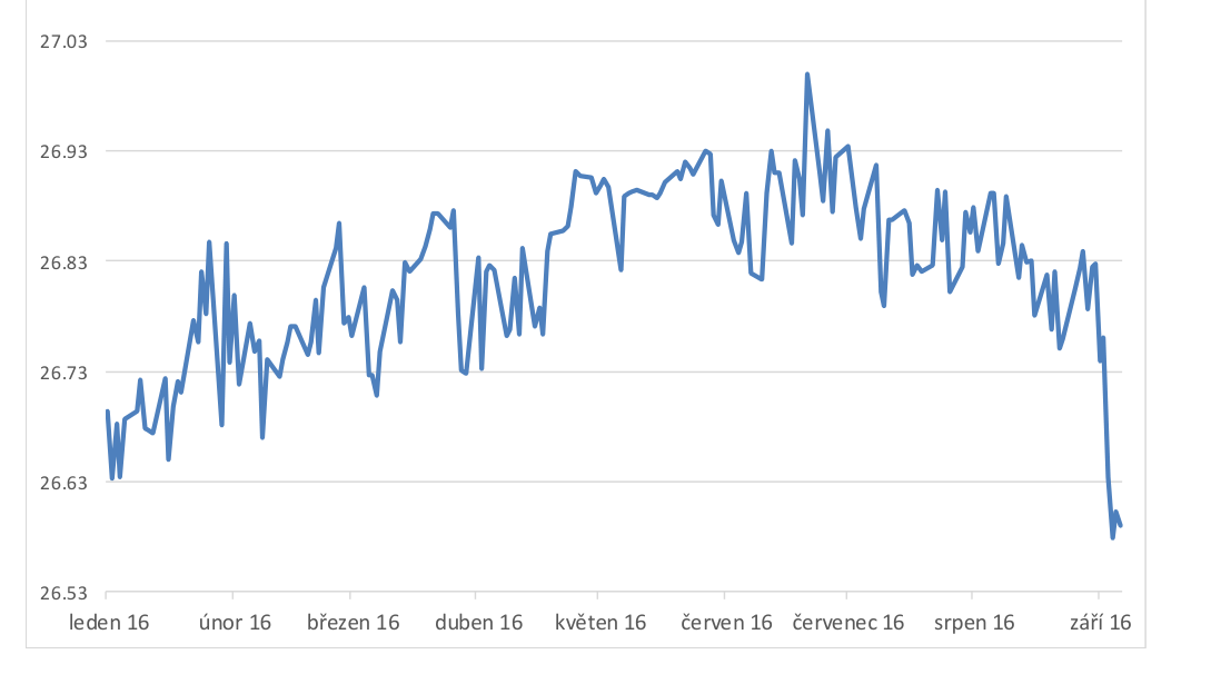
The expected appreciation is very small and stands out only in comparison with the even smaller additional appreciation at the two-year horizon, which at the beginning of September pointed somewhere toward 26.85. This year's path of the two-year forward is captured in Chart 5, which shows it hovering around 26.80 on average; in the first half of the year it tended to weaken, and in September, in reaction to the speculation, it strengthened to roughly 26.60. It was this strong a year ago as well, but after the speculation faded it gradually returned to 26.80, so it is quite possible that we will see a similar pattern this year too. My interpretation of the forward curve is that a certain segment of the market expects the floor to be abandoned immediately after the hard commitment expires, which also squares with anecdotal evidence.

The future appreciation implied by forwards is mild either because the market assumes only a slight move in the exchange rate after the commitment is abandoned, or because only a small share of market participants are speculating on its abandonment. The first of these hypotheses gains credibility from the fact that not even the two-year forward points to a marked appreciation of the koruna, not even during the September wave of speculation; and yet the overwhelming majority of market participants expect the exit to come within two years (see, for example, the September Financial Market Inflation Expectations survey). These market expectations measured by forward prices also correspond quite well to the average estimates of the nominal equilibrium exchange rate produced by the Monetary Department, which stand at 26.85 for the current quarter and 26.60 for the end of 2017.[7] They are not consistent, however, with the g3 model, which expects appreciation beyond the 26 CZK/EUR threshold; more precisely, they are not in line with the model's expectation of a steep rise in rates, which contributes to a stronger koruna over the forecast horizon.

5. Specific comments and questions on the Report

The wage bill in real terms grew noticeably faster year on year in the second quarter than consumption did (5.6% versus 2.2%). Can this difference be partly explained by the permanent income hypothesis? The g3 model itself, unlike, for example, the core model of the Ministry of Finance, does not assume the existence of consumers who would spend a fixed share of their current income (so-called rule-of-thumb consumers, who either do not optimize consumption or cannot smooth it because of credit constraints). The available empirical literature shows that g3 is specified correctly in this respect, because the permanent income hypothesis is a reasonable first approximation of actual consumer behavior (Havranek and Sokolova, 2016).
Like this opinion, the Report equates the forward/futures curve with the market outlook for prices, but for commodities instead of the exchange rate. For commodities, though, the unbiasedness hypothesis does not hold. The futures curve does of course contain an element of prediction of the future spot price, but it is strongly influenced by the following factors: 1) storage and insurance costs, 2) the so-called convenience yield, 3) other physical properties of the commodity, and 4) hedging demand from producers of the commodity exceeding hedging demand from buyers of the commodity (which is Keynes's explanation of backwardation), which makes futures prices understate future spot prices.
I appreciate the work on the box on the effect of the number of working days on GDP growth, which in the end was not included in the Report. If the Monetary Department is considering incorporating calendar effects into the forecast, I would argue for an adjustment technique that is not linear but allows a declining marginal effect of additional days beyond the quarterly average.

In other words, if the first quarter has one working day more than the average while the second has three days more than the average, I would expect the size of the adjustment for the second quarter to be less than three times the adjustment for the first. The reason is that consumption and the amount of work done will be affected not only by the number of hours worked but also by regular monthly payments and deadlines.

Retail sales and industrial production fell year on year in July. I would like to know why the seasonal adjustment method has, at first sight, a larger effect on sales (after adjustment practically at the level of the HP trend, the swing almost fully smoothed out) than on industrial production (deep below the HP trend); see appendices 9 and 10 of the Report. The year-on-year drop in industrial production, even in seasonally adjusted terms, was the sharpest in 80 months in July. It is unlikely that plant-wide holidays can explain this whole decline. What does the statement that they explain it "to a considerable extent" (p. 2) mean? It should be possible to estimate this effect, much as is done for the calendar adjustment.
I see a certain inconsistency in the forecast taking its USD/EUR projection from Consensus Forecast while using the futures curve for the oil price projection (described on p. 7 of the Report). As I have already mentioned, currency forwards are actually traded contracts, so it makes sense to trust them more than analysts' estimates. The unbiasedness hypothesis, by contrast, does not hold for commodities, so I would expect the two data sources to be used the other way around for these projections.
I am not sure the Report needs to devote so much space to PRIBOR, when it is essentially not a traded rate and its relevance in the current situation is unclear. The space saved could be used to discuss, for example, implied rates (see section 3 of this opinion), which until now have usually received only a brief mention in the MPD.
With the exit approaching, I would welcome analyses in the Report comparing the growth of the CNB and ECB balance sheets since the launch of the exchange rate commitment and the potential implications for the future path of the koruna (for example in the form of a non-public box). I would also welcome greater use and interpretation of the forward curve of the exchange rate (see section 4 of this opinion).
In the second chart in appendix 12 (the interest rate differential), the legend is mislabeled. The chart also illustrates what I consider an unrealistic assumption of the forecast, the rise of the differential to as much as 2.5%, which is probably driven by the assumption of a higher neutral interest rate in the Czech Republic than in the euro area, where the neutral rate is, according to the best available evidence (Holston et al., 2016), now negative, as the market outlook for Euribor reflects.

References

Dvorak, M., Komarek, L., Komarkova, Z., Ters, K., and Urban, Y. (2016): "Longer Term Yield Decomposition: An Analysis of the Czech Government Yield Curve," ongoing CNB research project C7/16.
Fama, E. (1984): "Forward and Spot Exchange Rates," Journal of Monetary Economics 14, 319-38.
Havranek, T., Sokolova, A. (2016): "Do Consumers Really Follow a Rule of Thumb? Three Thousand Estimates from 130 Studies Say 'Probably Not'," CNB working paper, not yet refereed.
Holston, K., Laubach, T., and Williams, J. (2016): "Measuring the Natural Rate of Interest: International Trends and Determinants," FRBSF Working Paper 2016-11.
Krippner, L. (2015): "A Comment on Wu and Xia and the Case for Two-Factor Shadow Short Rates," CAMA
Working Paper 48/2015.
Nelson, C. and Siegel, A. (1987): "Parsimonious modelling of yield curves," Journal of Business 60(4), 473-489.
Wu, J. and Xia, F. (2016): "Measuring the Macroeconomic Impact of Monetary Policy at the Zero Lower Bound,"
Journal of Money, Credit, and Banking, 48(2-3), 253-291.

Notes

[1] I thank Marek Rusnak for help with the Matlab code for computing the shadow rate, Michal Dvorak for constructing and updating the data for that computation and for repeated consultations, Wu Jing (University of Chicago) for sending the code and instructions, Petr Frydrych and Vlastimil Cadek for discussion of implied yields, Martin Motl for providing the equilibrium exchange rate estimates, Vaclav Hausenblas for help with the data in the section on forward rates, and Jiri Schwarz, Michal Franta, and Michal Hlavacek for discussion of forwards. This opinion of course reflects my own interpretation of the data, the estimates, and the discussions with colleagues.

[2] Using them, though, would require lowering the effective lower bound. A leading expert on negative rate policy, Miles Kimball (University of Colorado), will give a seminar and a mini-course on this topic at the CNB (November 10 and 11).

[3] In the opinion on Situation Report No. 1 of 2016, Michal Franta also argues convincingly that estimates based on the yield curve are conceptually more appropriate for the purposes of the g3 model than the extrapolation from NiGEM.

[4] More precisely, a credible calculation of the rates by this method would take several months of work. Wu Jing is also willing, if there is interest, to come to the CNB and give a seminar or a mini-course on shadow rates.

[5] The advantage of comparing two shadow rates instead of one shadow and one "official" rate is that what matters is not the absolute level at which a given technique puts the shadow rate (whether that is −2% or −8%) but only the difference in level between the two countries. Krippner (2015) also shows that his method is ordinally robust, so I trust the result that the ECB shadow rate is not currently lower than the CNB shadow rate.

[6] The discontinuity of the forward curve at the beginning of the year is not driven by the balance sheet effect, since that causes only a temporary, not a persistent, decline in the price of the forward. These temporary swings can indeed be observed in the data, very clearly for the two-year forward, for example. I also grant that liquidity in forward contracts with maturities over 1 year is noticeably lower, but they are still traded contracts, as can be seen, for example, from the trade repositories under the EMIR regulation.

[7] It must be said, though, that the individual methods for computing the equilibrium exchange rate give considerably different results.