How to Solve the Price Puzzle? A Meta-Analysis
Marek Rusnak, Tomas Havranek, & Roman Horvath (2013), "How to Solve the Price Puzzle? A Meta-Analysis." Journal of Money, Credit and Banking 45(1), 37-70. https://doi.org/10.1111/j.1538-4616.2012.00561.x.
MAREK RUSNAK, TOMAS HAVRANEK, and ROMAN HORVATH
MAREK RUSNAK AND TOMAS HAVRANEK are at Czech National Bank, Economic Research Department, and Charles University, Institute of Economic Studies (E-mails: marek.rusnak@cnb.cz and tomas.havranek@cnb.cz, respectively). ROMAN HORVATH is at Charles University, Institute of Economic Studies (E-mail: roman.horvath@gmail.com).
Received February 14, 2011; and accepted in revised form April 12, 2012.
JEL codes: C83, E52
* We are grateful to Adam Elbourne, Bill Gavin, Jakob de Haan, Tomas Holub, Sergey Slobodyan, Tom Stanley, Harald Uhlig, and two anonymous referees for providing data or comments on previous versions of the manuscript. The paper benefited from discussions at the Meta-Analysis of Economics Research Colloquium 2010, Conway; the Scottish Economics Society Annual Conference 2011, Perth; the International Conference on Macro-economic Analysis and International Finance 2011, Rethymno; and the Annual Congress of the European Economic Association 2011, Oslo. All remaining errors are ours. We acknowledge financial support from the Czech Science Foundation (grant #P402/11/1487) and the Grant Agency of Charles University (grant #267011). The views expressed here are ours and not necessarily those of our institutions. An online appendix is available at http://meta-analysis.cz/price_puzzle.
Abstract
The short-run increase in prices following an unexpected tightening of monetary policy constitutes a puzzle frequently reported in empirical studies. Yet the puzzle is easy to explain away when all published models are quantitatively reviewed. We collect and examine about 1,000 point estimates of impulse responses from 70 articles that use vector autoregressions to study monetary transmission in various countries. We find that the puzzle is created by model misspecifications: especially by the omission of commodity prices, neglect of potential output, and reliance on recursive identification. Our results also suggest that the strength of monetary policy depends on the country’s openness, phase of the economic cycle, and degree of central bank independence.
Keywords: monetary policy transmission, vector autoregressions, price puzzle, meta-analysis.
How does monetary policy affect the price level? This fundamental question of monetary economics still ranks among the most controversial when it comes to empirical evidence. Although intuition and stylized macro models suggest that prices should decrease following a surprise increase in interest rates, empirical findings often challenge the theory. About 50% of modern studies using vector autoregressions (VARs) to investigate the effects of monetary policy report that after a tightening prices actually increase—at least in the short run. Beginning with Sims (1992), many different solutions to the “price puzzle” have been proposed, varying from alleged misspecifications of VARs (Giordani 2004, Bernanke, Boivin, and Eliasz 2005) to theoretical models that try to justify the observed rise in prices (Barth and Ramey 2002, Rabanal 2007).
Depending on the point of view, the price puzzle casts serious doubt on either the ability of VAR models to correctly identify monetary policy shocks or the ability of central banks to control inflation in the short run, or both. Since macroeconomists have produced a plethora of empirical research on the topic, it seems natural to ask what general effect the literature implies. The method designed to answer such questions is meta-analysis, a quantitative method of research synthesis commonly used in economics (Smith and Huang 1995, Stanley 2001, Disdier and Head 2008, Card, Kluve, and Weber 2010, Chetty et al. 2011). In contrast to narrative literature surveys, meta-analysis takes into account possible publication selection: the preference of authors, editors, or referees for results that are statistically significant or consistent with the theory, a bias that has become a great concern in empirical economic research (DeLong and Lang 1992, Card and Krueger 1995, Ashenfelter and Greenstone 2004, Havranek and Irsova 2011).
Meta-analysis enables researchers to examine the systematic dependencies of reported results on study design and to separate the wheat from the chaff by filtering out the effects of misspecifications. Meta-analysis can create a synthetic study with ideal parameters, such as the maximum breadth of data or a consensus best-practice methodology and, in our case, estimate the underlying effect of monetary policy corrected for misspecification and other biases. Furthermore, meta-analysis makes it possible to investigate how the strength of monetary transmission depends on the characteristics of the countries examined. In this paper, we attempt to collect all published studies examining monetary transmission within a VAR framework and extract point estimates of impulse responses together with the corresponding confidence bounds. We investigate the degree of publication selection, the role of model misspecification for the occurrence of the price puzzle, and the factors underlying the heterogeneity of price responses to monetary shocks across countries and over time.
Based on the mixed-effects multilevel model we illustrate how meta-analysis is able to disentangle various factors causing researchers to encounter the price puzzle. We show that when best practice is followed, the researcher is likely to find that prices decrease significantly soon after a tightening of monetary policy. Our results thus suggest that the puzzle stems from model misspecification rather than from what really happens in the economy. In addition, the results indicate publication selection in favor of the negative responses of prices to a monetary contraction. Finally, our analysis of the determinants of transmission heterogeneity suggests that monetary policy has a stronger effect on prices in more open economies, in countries with a more independent central bank, and during economic downturns.
The remainder of the paper has the following structure. Section 1 describes how we collected the estimates from VAR models. Section 2 reviews the suggested solutions to the price puzzle. Section 3 tests for publication selection bias and for the underlying effect of monetary tightening on prices. Section 4 examines the method and structural heterogeneity among impulse responses. Section 5 concludes. Appendix A provides additional robustness checks, and Appendix B lists the studies used to construct the data set.
1. THE IMPULSE RESPONSES DATA SET
Ever since the seminal contribution of Sims (1980), VARs have been the dominant empirical tool for investigating monetary transmission. Researchers using VARs to examine the impact of monetary policy usually assume that the economy can be described by the following dynamic model:
where is a vector of endogenous variables typically containing a measure of output, prices, interest rates, and, in the case of a small open economy, the exchange rate. Matrix describes contemporaneous relationships between endogenous variables, is a matrix lag polynomial, and is a vector of structural shocks with the variance–covariance matrix . The system is called the structural-form VAR. In order to estimate it, researchers rewrite the system to its reduced form:
where the elements of matrix are the convolutions of the elements of matrices and , and is a vector of reduced-form shocks with the variance–covariance matrix ; the relationship between structural shocks and reduced-form residuals is . The dynamic responses of endogenous variables to structural shocks are described by impulse response functions.
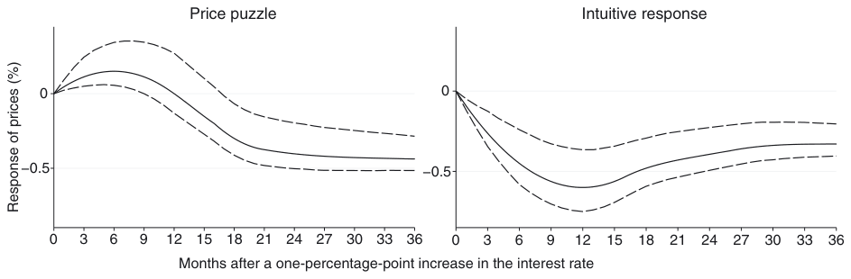
Figure 1 presents two stylized types of the price level’s impulse responses to a monetary tightening. The left panel demonstrates the price puzzle: prices increase significantly in the short run. In contrast, the right panel shows a response that corresponds with the mainstream prior: the price level declines soon after a tightening.
The first step of meta-analysis is to select the studies to be included. While some meta-analysts use both published and unpublished studies, others confine their sample to journal articles (e.g., Abreu, de Groot, and Florax 2005). Including working papers and mimeographs in meta-analysis does not help alleviate publication bias: if journals systematically prefer certain results, rational authors will already adopt the same preference in the earlier stages of research as they prepare for journal submission. Indeed, empirical evidence suggests no difference in the magnitude of publication bias between published and unpublished studies (see the meta-analysis of 87 meta-analyses by Doucouliagos and Stanley Forthcoming). Even if there was a difference, modern meta-regression methods not only identify but also filter out the bias. Therefore, as a preliminary and simple criterion of quality, we only consider articles published in peer-reviewed journals or in handbooks (such as the Handbook of Macroeconomics).
The following literature search strategy was employed. First, we examined two narrative surveys (Stock and Watson 2001, Egert and MacDonald 2009) and set up a search query able to capture most of the relevant studies; we searched both the EconLit and RePEc databases. Next, we checked the references of studies published in 2010 and the citations of the most widely cited study in the VAR literature (Christiano, Eichenbaum, and Evans 1999). After going through the abstracts of all the identified studies, we selected 195 that showed any promise of containing empirical estimates of impulse responses and examined them in detail. The search was terminated on September 15, 2010.
To be able to use meta-analysis methods fully, we exclude the studies that omit to report confidence intervals around impulse responses. Unfortunately, we thus have to exclude some seminal articles such as Sims (1992) or a few recent studies that estimate time-varying parameter VARs. To obtain a more homogeneous sample we only focus on studies that define a monetary policy shock as a shock in the interest rate. A number of studies investigate the change in the monetary base; since Bernanke and Blinder (1992) and Sims (1992), however, the majority of the literature investigates interest rate shocks because most central banks now use the interest rate as their main policy instrument. We only include studies examining the response of the price level; a minority of studies examine the responses of the inflation rate. These inclusion criteria leave 70 studies in our database. The full list of studies included in the data set can be found in Appendix B, and the list of excluded studies is presented in the online appendix at http://meta-analysis.cz/price_puzzle.
Considering the richness and heterogeneity of the empirical evidence on the effects of monetary policy, it is surprising there has been no quantitative synthesis using modern meta-regression methods.1 One reason is that the results are typically presented in the form of graphs instead of numerical values, and the graphs contain estimates for many time horizons following the monetary policy shock. Researchers usually investigate up to 36- or 48-month horizons when using monthly data and up to 20 quarters when using quarterly data; it is unclear which horizon should be chosen to summarize the effect.
Our meta-analysis is designed in the following way. We extract responses at 3- and 6-month horizons to capture the short-run effect, at 12- and 18-month horizons to capture the medium-run effect, and at the 36-month horizon to capture the long-run effect. We enlarge the graphs of impulse responses and using pixel coordinates we measure the response and its confidence bounds. The graphs of all impulse responses as well as the extracted values are available in the online appendix. The resulting measurement error is random, similar to the rounding error in numerical outcomes, and thus inevitable in a meta-analysis.
The extracted values must be transformed into a common metric to ensure that the estimates are comparable. To standardize the estimates so as they represent the effect of a 1 percentage point increase in the interest rate, we divide the responses by the magnitude of the monetary policy shock used in the study. (When we were uncertain about the magnitude of shock used in the primary study, we contacted the authors.) In the case of factor-augmented VAR (FAVAR) studies, where the responses are usually given in standard deviation units, we normalize the responses by the standard deviation of the particular time series.
Since the confidence intervals around the estimates of impulse responses are often asymmetrical (confidence intervals are usually computed by the Bayesian Monte Carlo integration method; see Sims and Zha 1999), the standard errors of the estimates cannot be obtained directly. In this case we approximate the standard error by the distance from the point estimate to the confidence bound closer to zero; that is, we take the lower confidence bound for positive responses and the upper bound for negative responses. This bound determines significance and would be associated with potential publication selection. Should we use the average of the distance to both confidence bounds, the inference would remain similar; these additional results are available in the online appendix. When the reported confidence interval is presented in standard deviation units (e.g., two standard deviations on both sides), we can immediately approximate the standard error. Otherwise, we proceed as if the estimates were symmetrically distributed and assume that, for example, the 68% confidence interval represents an interval of one standard error around the mean.
Following the recent trend in meta-analysis (Disdier and Head 2008, Havranek and Irsova 2011), we use all reported estimates from the 70 primary studies. Arbitrarily selecting the “best” estimate or using the average reported estimate would discard a great deal of useful information about the differences in methods within one study.
The number of impulse responses collected for each of the horizons is approximately 210, which in total amounts to more than 1,000 point estimates. More specifically, we collect 208 estimates for the 3-month horizon, 215 for the 6- and 12-month horizons, 217 for the 18-month horizon, and 205 for the 36-month horizon. For comparison, consider Nelson and Kennedy (2009), who review 140 economic meta-analyses and report that the median analysis only uses 92 point estimates from 33 primary studies. The oldest study in our sample was published in 1992 and the median study was published in 2006; the data set covers evidence from 31 countries, and we build upon the work of 103 researchers that produced the impulse responses. The median time span of the data used by the primary studies is 1980–2002. All studies in the sample combined receive approximately 800 citations in Google Scholar per year, indicating the influence of VARs in monetary economics.
| Methodology used in the estimation | |||||||
|---|---|---|---|---|---|---|---|
| All | Commodity | Trend/gap | FAVAR | SVAR | Sign | Single | |
| No. of responses estimated | 208 | 125 | 33 | 11 | 60 | 31 | 64 |
| Price puzzle present | 104 | 61 | 8 | 8 | 20 | 3 | 24 |
| Price puzzle significant | 32 | 16 | 1 | 3 | 6 | 0 | 5 |
NOTES: Commodity = commodity prices are included in the VAR; Trend/gap = time trend or output gap is included; FAVAR = a factor-augmented VAR is estimated; SVAR = nonrecursive identification is used; Sign = shocks are identified by imposing sign restrictions; Single = the VAR is estimated on the sample containing a single monetary policy regime.
2. COLLECTING THE PIECES OF THE PUZZLE
To motivate the selection of explanatory variables in the multivariate meta-regression analysis (Section 4), we now briefly review the methodological solutions to the price puzzle that have been proposed in the literature. Most of these remedies have proven to alleviate the puzzle in some cases; none of them, though, has been fully successful in solving it. Table 1 demonstrates that from the 208 estimates collected for the 3-month horizon, exactly half exhibit the price puzzle, and in 15% of the estimates the puzzle is even statistically significant at the 5% level. The table summarizes the effectiveness of the different solutions to the puzzle. Even in the case of the most effective solution, 24% of specifications still exhibit the puzzle (except for sign restrictions, which in some cases represent a tautological solution). Clearly no single misspecification is responsible for the price puzzle. But perhaps the puzzle is associated with a combination of bad method choices. In the following paragraphs we describe why some methods are thought to be better than others and what may help explain the reported puzzle.
2.1 Omitted Variables
Commodity prices.
According to Sims (1992), researchers observe the price puzzle because central banks are forward looking and react to the anticipated future movements of inflation by raising the interest rate. When researchers omit information about future inflation in their VAR system, the examined shocks become combinations of true monetary policy shocks and endogenous reactions to expected inflation. If the central bank does not fully accommodate the expected inflation, the data show that an increase in the interest rate, mistakenly recognized as a monetary policy shock, is followed by an increase in the price level. Sims (1992) finds that including commodity prices in the VAR mitigates the price puzzle. Nevertheless, the evidence from the entire literature summarized in Table 1 suggests that the inclusion of commodity prices helps little by itself. Almost 50% of VAR models with commodity prices still report the puzzle.
Output gap.
Giordani (2004) argues that the use of GDP in the VAR system without controlling for the potential output of the economy can bias the estimates and cause the price puzzle. He claims that the inclusion of commodity prices alleviates the puzzle mostly because commodity prices contain useful information about the output gap, not just because they are a good predictor of future inflation. Indeed, Hanson (2004) finds little correlation between the ability to solve the price puzzle and the ability to forecast inflation. Approximately 16% of the studies in our sample use the output gap (or add a time trend), but some of them still find the puzzle.
Factor-augmented VAR.
To address the major shortcomings of standard small-scale VARs, Bernanke et al. (2005) introduce the factor-augmented VAR approach. They argue that policymakers take into account hundreds of variables when deciding about monetary policy. Standard VAR models with three to six variables may therefore suffer from omitted variable bias. The FAVAR approach, on the other hand, makes use of additional information by extracting principal components from many time series and, as Bernanke et al. (2005) argue, should solve the price puzzle. But evidence from the literature (Table 1) indicates that FAVAR is ineffective in explaining the puzzle away.
2.2 Identification
While some researchers stress the role of omitted variables, others argue that the puzzle arises from implausible identification of monetary policy shocks. The usual recursive identification, which assumes that monetary policy affects output and prices only with a lag, is, for example, not consistent with the New Keynesian class of theoretical models (Carlstrom, Fuerst, and Paustian 2009).
Nonrecursive identification.
The main idea of a nonrecursive identification of shocks, going back to Bernanke (1986) and Blanchard and Watson (1986), is that the matrix contemporaneously linking structural shocks and reduced form residuals is no longer lower triangular, but that it assumes a general form indicated by theory: the rows of the matrix have a structural interpretation. The restrictions presented by Kim and Roubini (2000), for example, are elicited from the structural stochastic equilibrium model developed by Sims and Zha (1998). Although nonrecursive identification is theory consistent, Table 1 suggests that in almost 33% of the responses computed using this strategy the price puzzle still occurs.
Sign restrictions.
Canova and Nicolo (2002) and Uhlig (2005) present a novel identification approach that assigns a structural interpretation to orthogonal innovations by imposing sign restrictions on the responses to shocks. The method is attractive since sign restrictions can be derived directly from structural theoretical models. The identifying assumptions are clearly stated and the shocks can be given the structural interpretation without imposing zero restrictions. As Table 1 documents, VARs estimated with sign restrictions rarely encounter the price puzzle.
2.3 Monetary Policy Regime
Another stream of literature suggests that the price puzzle is historically limited to periods of passive monetary policy or that it emerges when researchers mix data for different monetary policy regimes (Elbourne and de Haan 2006, Borys, Horvath, and Franta 2009). For example, if a researcher assumes that the central bank uses the interest rate to target inflation, although for some part of the sample monetary or exchange rate targeting was in place, monetary policy shocks in the VAR system become incorrectly identified. Table 1 shows that most researchers who evaluate monetary transmission in a period of a single monetary policy regime do not report the price puzzle.
The previous paragraphs illustrate that the quality of studies included in our sample varies. Some of the studies are obviously misspecified. Will not the misspecified studies bias the research synthesis? Indeed, this has been an objection to meta-analysis, and an alternative approach called best-evidence synthesis has been proposed (Slavin 1986). Proponents of best-evidence synthesis argue that we should not include bad studies when we are interested in the average effect. If misspecifications have a systematic influence on the results, then the simple average produced by meta-analysis will be biased. The problem with best-evidence synthesis is the definition of best evidence. For example, should we discard all VAR models that omit commodity prices? In that case we would have 125 observations for the 3-month horizon. But if we additionally threw away all studies that neglect potential output, mix monetary policy regimes, and resort to recursive identification, we would be left with a handful of observations.
The empirical literature on monetary transmission is rich in method choices that the researcher must make. When more and more aspects of methodology become a subject of scrutiny, best-evidence synthesis boils down to selecting the best study from the literature. But this denies the purpose of research synthesis—to provide robust results and explain the differences between the findings of individual studies. Meta-analysis, in contrast, enables us to test explicitly whether misspecifications of primary studies affect the reported results in a systematic way. If so, we can define what we think constitutes best practice and estimate the average impulse response conditional on such best practice without throwing away any information. Because best practice is subjective, we will try several alternative definitions. Moreover, we want to explain what makes researchers report the price puzzle. If misspecifications cause the price puzzle, we need misspecified studies as well.
3. CONSEQUENCES OF PUBLICATION SELECTION
After we have collected about 1,000 estimates of the response of prices to monetary tightening, a natural question arises: what general impulse response does the literature suggest? Meta-analysis was originally developed in medicine to combine many small studies into a large one, and therefore to boost the number of degrees of freedom. Clinical trials are costly, and meta-analysis thus became the dominant method of taking stock of medical research. Estimating a VAR model may be less expensive, but the degrees of freedom in macroeconomics are limited. Hence, the original purpose of meta-analysis is useful even here since it combines information from many countries and time periods: when recomputed into quarters the primary studies in our sample taken together use 2,452 unique observations.
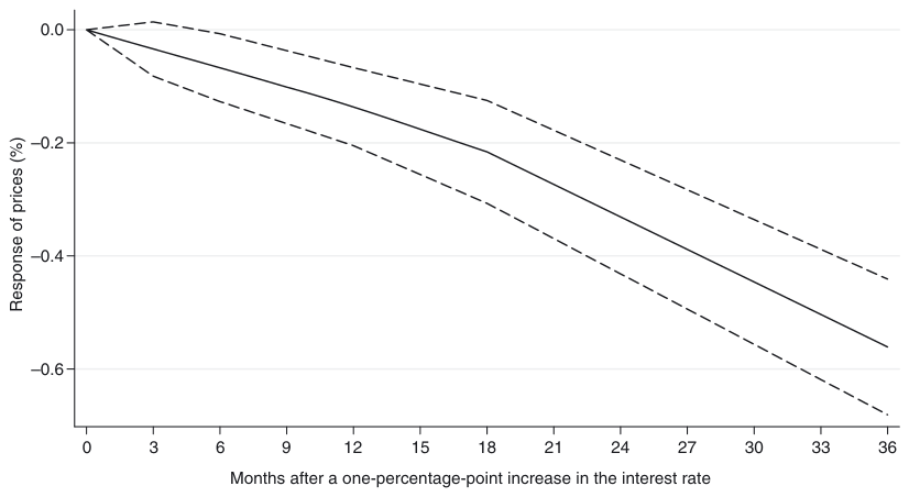
Taking a simple mean of all point estimates for each of the five horizons implies the impulse response function depicted in Figure 2. This average impulse response shows a relatively intuitive short-run reaction of prices to a 1 percentage point increase in the interest rate: prices decline already in the short run, the decrease becomes significant in the medium run and reaches 0.56% after 36 months. Nevertheless, the response shows no sign of bottoming out.
Simply averaging the collected impulse responses has two major shortcomings. First, it ignores possible publication selection. If some results are more likely to get published than others, the average becomes a biased estimator of the underlying impulse response. Second, it ignores heterogeneity in the results of the primary studies. Since different researchers use different data and methods, and the studies are of different quality, it is unrealistic to assume that all estimates are drawn from the same population. In addition, as discussed in Section 2, some VAR models are misspecified, and if misspecifications have a systematic influence on the results, it is possible to improve upon the average response by filtering out the misspecifications. We address publication selection in this section and heterogeneity and misspecification issues in Section 4.
Stanley (2008), among others, points out that publication selection is of major concern for empirical research in economics. When there is little theory competition for what sign the underlying effect should have, estimates inconsistent with the predominant theory will be treated with suspicion or even be discarded. An illustrative example can be found in the literature on the effect of a common currency on trade (Rose and Stanley 2005): it is hard to defend negative estimates of the trade effect of currency unions. The negative estimates most likely result from misspecification, and researchers may be correct in not stressing them. On the other hand, it is far more difficult to identify excessively large estimates of the same effect that also arise from misspecifications. No specific threshold exists above which the estimate would become suspicious. If researchers include the large positive estimates but omit the negative ones, the inference will be on average biased toward a stronger effect.
A similar selection, perhaps of lower intensity, may be taking place in the VAR literature on monetary transmission as well (Uhlig 2010, p. 17, provides anecdotal evidence).2 Some researchers treat the price puzzle as a clear indication of a misspecification error and try to find an intuitive impulse response for interpretation. Statistical significance is also important. Significant impulse responses are more convenient for interpretation, and especially researchers in central banks may be interested in reporting a well-functioning monetary transmission with a significant reaction of prices to a change in monetary policy. The selection for significance does not distort the average estimate from the literature if the true underlying effect equals zero, but otherwise it creates a bias, again in favor of a stronger effect, since estimates with the wrong sign are less likely to be significant.
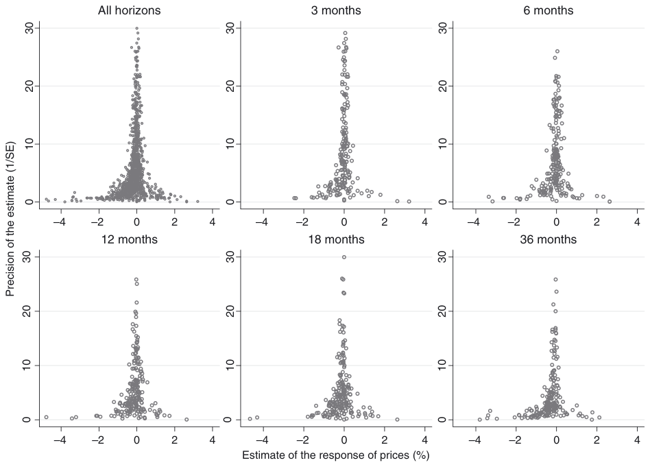
A common way to detect publication selection is an informal examination of a so-called funnel plot (Stanley and Doucouliagos 2010). The funnel plot depicts the estimates on the horizontal axis against their precision (the inverse of the standard error) on the vertical axis. If there is no heterogeneity or misspecification, the estimates with the highest precision will be close to the true underlying effect. In the absence of publication selection the funnel is symmetrical: the reported estimates are dispersed randomly around the true effect. The asymmetry of the funnel plot suggests publication bias; for example, if estimates with a positive sign are less likely to be selected for publication, estimates on the right side of the funnel will be underrepresented.
The funnel plots for all five horizons are depicted in Figure 3. The plots resemble funnels commonly reported in economic meta-analyses, which indicates that the employed approximation of standard errors is plausible. As expected, the left part of all funnels is clearly heavier, suggesting publication selection against the price puzzle and in favor of the more negative (i.e., stronger) effects of monetary tightening on prices. Nevertheless, the interpretation of funnel plots is subjective, and we need a more formal test of publication bias.
Given small samples, authors wishing to obtain significant results may be tempted to try different specifications until they find estimates large enough to offset the standard errors. In contrast, with large samples even tiny estimates might be statistically significant, and authors therefore have fewer incentives to conduct a specification search. If publication selection is present, we should observe a relationship between an estimate and its standard error (or the square root of the number of observations). The following regression formalizes the idea (Card and Krueger 1995):
where denotes the true underlying effect, denotes the effect’s th estimate, denotes the magnitude of publication bias, denotes the standard error of , and denotes a disturbance term.
Specification (3) has become the cornerstone of modern meta-analysis in medicine and the social sciences, including economics. The question is whether the method is suitable for summarizing graphical results such as impulse responses. In order for this meta-analysis method to be valid, the distribution of empirical effects needs to be symmetrical in the absence of publication bias (usually it is assumed that the disturbance term in (3) is normally distributed). But impulse responses are nonlinear functions of the coefficients estimated in the VAR system; as discussed in Section 1, the confidence intervals around the individual estimates are often asymmetrical. If the pattern of asymmetry is not random across the individual estimates, the distribution of the impulse responses will not be symmetrical even in the absence of publication bias, and the test for publication bias will be invalid.
Systematic asymmetry of the distribution of impulse responses would manifest as a significant difference between the average distance from the point estimate of the impulse response to the lower and upper confidence bound. We select the 68% confidence bound (34% on both sides of the estimate), which for a symmetrical distribution would imply a distance of one standard error on both sides of the mean. The difference of the distances is significant at the 5% level for only one of five horizons (the 12-month horizon), and even there the difference is small: the average lower confidence interval is 11.6% farther from the mean than is the average upper confidence interval. It is unlikely that such a small difference could explain the degree of asymmetry apparent from Figure 3. It cannot explain the asymmetry of the collected point estimates of the impulse responses at the 12-month horizon, where the distance from the 16th percentile to the mean is 53.1% larger than the distance from the mean to the 84th percentile. For this reason, we employ the standard meta-analysis methodology—bearing in mind that the results concerning publication bias must be interpreted with some caution.3
In practice, meta-analysts rarely estimate specification (3) directly since it suffers from heteroskedasticity by definition (the explanatory variable is a sample estimate of the standard deviation of the response variable). Instead, weighted least squares are used to gain efficiency, and they require that specification (3) be divided by , the measure of heteroscedasticity (Stanley 2008):
where denotes the approximated -statistic of the estimate and the new disturbance term has constant variance. Note that the intercept and the slope are now reversed: the slope measures the true effect and the intercept measures publication bias. In addition to removing heteroskedasticity, specification (4) gives more weight to more precise results, which represents a common approach in meta-analysis. Testing the significance of in this specification is analogous to testing the asymmetry of the funnel plot—it follows from rotating the funnel plot and dividing the values on the new vertical axis by . Testing the significance of constitutes a test for the true underlying effect of monetary tightening on prices, corrected for publication selection.
The intercept of specification (4), which in our case measures the degree of publication bias, has an alternative interpretation that is sometimes used in economics meta-analyses. Since the response variable is the -statistic, the intercept represents the average -statistic that the literature reports for the effect in question. The average is, however, conditional on precision (i.e., the inverse of standard error). If precision was not included in specification (4), such as, for example, in the meta-analysis by Görg and Strobl (2001), the intercept would represent the unconditional average -statistic. In that case, however, publication bias could not be separated from the true effect.
Our specification controls for precision, which means that the intercept corresponds to the average -statistic conditional on precision being close to zero (or, alternatively, on the standard error of the estimated coefficient being close to infinity). The true effect has no relation to the observed -statistic as precision goes to zero; in other words, the precision term in (4) filters out any underlying effect. When precision is zero, the average -statistic should be zero as well. If it is not, something is wrong with the literature, and we observe signs of publication bias (or any other bias that causes the asymmetry of funnel plots). A more detailed treatment of this problem is available in Stanley (2008).
Since we use all reported impulse responses we need to account for the potential dependence of estimates within one study (Disdier and Head 2008); in such a case, (4) would be misspecified. As a remedy, researchers typically employ the mixed-effects multilevel model (Doucouliagos and Stanley 2009, Havranek and Irsova 2011):
where and denote estimate and study subscripts, respectively. The overall error term now consists of study-level random effects and estimate-level disturbances (), and its variance is additive since both components are assumed to be independent: , where denotes between-study variance and within-study variance. If approaches zero the benefit of using the mixed-effect estimator instead of ordinary least squares (OLS) dwindles. To put the magnitude of these variance terms into perspective the within-study correlation is useful: , which expresses the degree of dependence of estimates reported in the same study, or equivalently, the degree of between-study heterogeneity.
The mixed-effects multilevel model is analogous to the random-effects model commonly used in panel-data econometrics. We follow the terminology from multilevel data modeling, which calls the model “mixed effects” since it contains a fixed () as well as a random () part. For the purposes of meta-analysis the multilevel framework is more suitable because it takes into account the unbalancedness of the data (the restricted maximum likelihood estimator is used instead of generalized least squares), allows for nesting multiple random effects (study level, author level, or country level), and is thus more flexible (Nelson and Kennedy 2009).
The outcomes of the mixed-effects estimator are presented in Table 2. OLS with standard errors clustered at the study level are reported in Appendix A. Table A1 gives even more significant results for publication bias. The within-study correlation is large, indicating that the mixed-effects estimator is more appropriate, which is confirmed by likelihood-ratio tests.4 Compared to the simple average, the response of prices corrected for publication bias is more positive (i.e., weaker), corroborating evidence for publication selection in favor of the stronger responses of prices to monetary policy contraction. Moreover, the magnitude of publication bias increases with the time horizon after the shock. This result is in line with Doucouliagos and Stanley (Forthcoming), who find stronger publication selection for research questions with weaker theory competition. For the short run, some disagreement occurs regarding the effects of monetary policy on prices because of the cost channel. (Since firms depend on credit to finance production, their costs rise when the central bank increases the interest rate, and they may increase prices.) On the other hand, a consensus emerges about the long-run effect: prices should eventually decrease after monetary policy tightening; estimates showing the opposite would be difficult to publish.
| Mixed-effects multilevel | |||||
|---|---|---|---|---|---|
| Horizon | 3 months | 6 months | 12 months | 18 months | 36 months |
| Intercept (bias) | 0.058 | −0.088 | −0.176 | −0.325** | −0.806*** |
| (0.167) | (0.166) | (0.145) | (0.128) | (0.126) | |
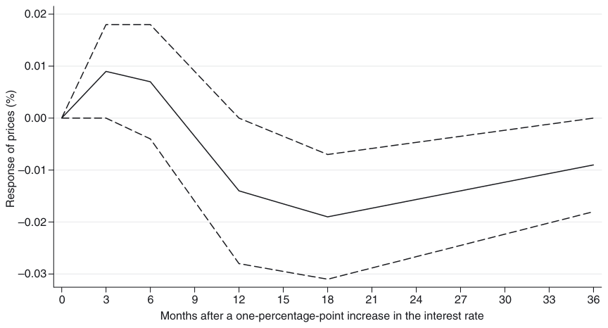
| 1/SE (effect) | 0.009 | 0.007 | −0.014 | −0.019 | −0.009 |
| (0.009) | (0.011) | (0.014) | (0.012) | (0.010) | |
| Within-study correlation | 0.43 | 0.56 | 0.46 | 0.41 | 0.14 |
| Observations | 208 | 215 | 215 | 217 | 205 |
| Studies | 69 | 70 | 70 | 70 | 63 |
Notes: Standard errors in parentheses. Response variable: the approximated -statistic of the estimate of the percentage response of prices to a 1 percentage point increase in the interest rate. *** and ** denote significance at the 1% and 5% levels, respectively.
The impulse response function corrected for publication bias is depicted in Figure 4: it exhibits the price puzzle. In the short run prices increase, but in the medium run they decrease and bottom out 18 months after the tightening. The maximum decrease in the price level, however, is negligible: only 0.02%. Compared to the average response reported in Figure 2, now the function shifts upward—especially in the long run, because publication bias is filtered out. Figure 4 would be our best estimate of the underlying impulse response if all heterogeneity between studies was random; the estimate is unconditional on the characteristics of the countries examined and on the methodology used. In the next section we relax the assumption of random heterogeneity and explain the differences in the reported estimates. In particular, we are interested in the average impulse response conditional on best-practice methodology.
Note: Confidence bands are constructed as +/− one standard error.
4. WHAT EXPLAINS HETEROGENEITY
As motivation for the empirical investigation of structural heterogeneity consider Figure 5, which depicts the differences in monetary transmission among selected countries. We use a simple random-effects meta-analysis to compute impulse-response functions. Simple meta-analysis weights each estimate by its precision and adds an estimate-specific random effect; it does not correct for publication bias. We use simple meta-analysis for estimation by countries since it requires fewer degrees of freedom than meta-regression. Figure 5 shows that the impulse responses for the United States, the United Kingdom, and Japan exhibit the price puzzle, but that monetary transmission in euro area countries seems to work intuitively and prices decline soon after a tightening. Nevertheless, a part of these differences may arise from the use of diverse methods since some countries are examined only in a few studies.
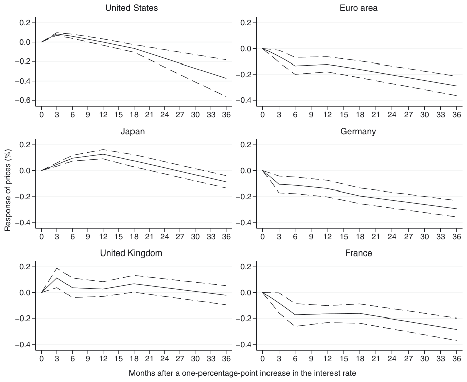
Note: Confidence bands are constructed as +/− one standard error.
To account for heterogeneity we extend the meta-regression (5) to the following multivariate version:
where denotes explanatory variables assumed to affect the reported estimates. The exogeneity assumptions become and .
Table 3 presents descriptions and summary statistics of all the explanatory variables we consider. In principle, they can be divided into five groups: variables capturing the fundamental characteristics of the economy (structural heterogeneity), data characteristics controlling for differences in the data used, specification characteristics controlling for differences in the basic design of the estimated models, estimation characteristics controlling for differences in econometric techniques, and publication characteristics controlling mainly for differences in quality not captured by other variables.
| Variable | Description | Mean | Std. dev. |
|---|---|---|---|
| Response (3M) | The percentage response of prices 3 months after a tightening | −0.034 | 0.692 |
| Response (6M) | The percentage response of prices 6 months after a tightening | −0.067 | 0.883 |
| Response (12M) | The percentage response of prices 12 months after a tightening | −0.136 | 1.012 |
| Response (18M) | The percentage response of prices 18 months after a tightening | −0.216 | 1.327 |
| Response (36M) | The percentage response of prices 36 months after a tightening | −0.561 | 1.714 |
| 1/SE | The precision of the estimate of the response (all horizons) | 6.805 | 7.821 |
| Structural heterogeneity | |||
| GDP per capita | The logarithm of the country's real GDP per capita | 9.881 | 0.414 |
| GDP growth | The average growth rate of the country's real GDP | 2.668 | 1.035 |
| Inflation | The average inflation of the country | 7.748 | 14.26 |
| Inflation volatility | The standard deviation of the difference between the country's inflation and its Hodrick-Prescott-filtered inflation trend | 6.234 | 33.43 |
| Financial development | The financial development of the country measured by (domestic credit to private sector)/GDP | 0.837 | 0.414 |
| Openness | The trade openness of the country measured by (exports + imports)/GDP | 0.460 | 0.401 |
| CB independence | A measure of central bank independence (Arnone et al. 2009) | 0.774 | 0.143 |
| Data characteristics | |||
| Monthly | = 1 if monthly data are used | 0.630 | 0.483 |
| Time span | The number of years of the data used in the estimation | 18.83 | 10.44 |
| No. of observations | The logarithm of the number of observations used | 4.889 | 0.675 |
| Average year | The average year of the data used (2000 as a base) | −8.926 | 7.881 |
| Specification characteristics | |||
| GDP deflator | = 1 if the GDP deflator is used instead of the consumer price index as a measure of prices | 0.177 | 0.382 |
| Single regime | = 1 if the VAR is estimated over a period of a single monetary policy regime | 0.296 | 0.457 |
| No. of lags | The number of lags in the model, normalized by frequency: lags/frequency | 0.610 | 0.370 |
| Commodity prices | = 1 if a commodity price index is included | 0.607 | 0.489 |
| Money | = 1 if a monetary aggregate is included | 0.529 | 0.499 |
| Foreign variables | = 1 if at least one foreign variable is included | 0.441 | 0.497 |
| Time trend | = 1 if a time trend is included | 0.126 | 0.332 |
| Seasonal | = 1 if seasonal dummies are included | 0.146 | 0.354 |
| No. of variables | The logarithm of the number of endogenous variables included in the VAR | 1.741 | 0.383 |
| Industrial production | = 1 if industrial production is used as a measure of economic activity | 0.430 | 0.495 |
| Output gap | = 1 if the output gap is used as a measure of economic activity | 0.028 | 0.165 |
| Other measures | = 1 if another measure of economic activity is used (employment, expenditures) | 0.119 | 0.324 |
| Variable | Description | Mean | Std. dev. |
|---|---|---|---|
| Estimation characteristics | |||
| BVAR | = 1 if a Bayesian VAR is estimated | 0.144 | 0.352 |
| FAVAR | = 1 if a factor-augmented VAR is estimated | 0.051 | 0.221 |
| SVAR | = 1 if nonrecursive identification is employed | 0.295 | 0.456 |
| Sign restrictions | = 1 if sign restrictions are employed | 0.144 | 0.352 |
| Publication characteristics | |||
| Study citations | The logarithm of [(Google Scholar citations of the study)/(age of the study) + 1] | 1.882 | 1.279 |
| Impact | The recursive RePEc impact factor of the outlet | 0.888 | 2.274 |
| Central banker | = 1 if at least one coauthor is affiliated with a central bank | 0.451 | 0.498 |
| Policymaker | = 1 if at least one coauthor is affiliated with a Ministry of Finance, IMF, OECD, or BIS | 0.055 | 0.228 |
| Native | = 1 if at least one coauthor is native to the investigated country | 0.446 | 0.497 |
| Publication year | The year of publication (2000 as a base) | 5.032 | 3.886 |
Structural heterogeneity
When constructing the variables that capture structural heterogeneity, we use the average values that correspond to the sample employed in the estimation of the impulse response. For instance, in the case of inflation: when the impulse response comes from a VAR model estimated on the 1990:1–1999:12 Italian data, we use the average inflation rate in Italy for the period 1990–1999. This approach increases the variability in regressors and describes the estimates more precisely than using the same year of structural variables for all extracted impulse responses. The variable GDP per capita reflects the importance of the degree of economic development of the economy for monetary transmission. To investigate whether the strength of transmission depends on the phase of the economic cycle, we include the variable GDP growth in the meta-regression. The underlying reason is related to credit market imperfections, which could amplify the propagation of monetary policy shocks during bust periods (Bernanke and Gertler 1989).
Next, we examine the variables implied by the various channels of the transmission mechanism. We include the trade openness of the economy to capture the importance of foreign developments for domestic monetary policy as well as the exchange rate channel of monetary transmission. Furthermore, as pointed out by Bernanke and Gertler (1995) and Cecchetti (1999), differences in financial structure may explain important portions of heterogeneity in monetary transmission. We include a measure of financial development approximated by the ratio of private credit to GDP.
We add the average level and volatility of inflation, as these may influence price setting behavior as well as monetary transmission (Angeloni et al. 2006). We expect that independent central banks are likely to be more credible (Rogoff 1985, Keefer and Stasavage 2003, Perino 2010). In consequence, economic subjects may respond more to monetary policy shocks. We test whether the degree of central bank independence affects the strength of monetary transmission.
Regarding the sources of the data, the trade openness, GDP growth, and GDP level per capita are obtained from Penn World Tables. The consumer price index, used to compute average inflation and inflation volatility, is obtained from the International Monetary Fund's International Financial Statistics. The ratio of domestic credit to GDP is obtained from the World Bank's World Development Indicators, and the index of central bank independence is extracted from Arnone et al. (2009).
Data characteristics
We control for the frequency of the data used in the VAR model: 63% of specifications use monthly data, the rest rely on quarterly data. To account for possible changes in transmission not explained by the structural variables (e.g., changes caused by globalization or financial innovations; see Boivin and Giannoni 2006), we include the average year of the sample period used in the estimation. Finally, we add the total number of observations to assess whether smaller samples yield systematically different outcomes.
Specification characteristics
To account for the different measures of the price level we include a dummy that equals one when the GDP deflator is used instead of the usual consumer price index (18% of specifications in primary studies). We add a dummy for the case where the data cover a period of a single monetary policy regime (30%). Next, we include the VAR's lag order normalized by the data frequency. We account for the cases where commodity prices, a money aggregate, foreign variables, a time trend, and seasonal dummies are included in the VAR. We also control for the number of endogenous variables in the model. Since the results might vary depending on the measure of economic activity, we introduce dummies for the cases where industrial production, the output gap, or another measure is used instead of GDP.
Estimation characteristics
Most of the studies in our sample estimate VAR models using the standard methods (OLS or maximum likelihood); we control for studies using Bayesian methods to address the problem of overparameterization (14% of specifications in primary studies) and for studies using the FAVAR approach to address the problem of omitted variables (5%). As for identification strategies, most of the studies employ recursive identification; we include a dummy for nonrecursive identification (30%) and a dummy for identification using sign restrictions (14%).
Publication characteristics
To proxy study quality we use the recursive RePEc impact factor of the outlet (because the journal coverage of RePEc is much more comprehensive than in other databases) and the number of Google Scholar citations of the study normalized by the study's age. We add a dummy for authors affiliated with a central bank and a dummy for authors working at policy-oriented institutions such as a Ministry of Finance, the International Monetary Fund, or the Bank for International Settlements. We include a dummy for the case where at least one co-author is “native” to the examined country: such authors may be more familiar with the data at hand, which could contribute positively to the quality of the analysis; on the other hand, such authors may have a vested interest in the results. We consider authors native if they either were born in the country or obtained an academic degree there. Finally, we use the year of publication to account for possible improvements in methodology that are otherwise difficult to codify.
In the first step, we estimate a general model containing all explanatory variables; the general model is not reported but is available in the online appendix. All variance inflation factors are lower than 10, indicating that the degree of multicollinearity is not too problematic. In the second step, we drop the variables which are for each horizon jointly insignificant at the 10% level.
For example, GDP per capita, the number of lags used, and most publication characteristics belong to the dropped variables. The insignificance of publication characteristics suggests that the quality of a given study is to a large extent captured by the methods used.
The resulting model is presented in Table 4. The specifications reported in this section are based on the mixed-effects multilevel estimator, but the inference would be similar from an OLS with standard errors clustered at the study level; these robustness checks are available in Appendix A. The similarity between the outcomes of these two estimators indicates that the exogeneity assumptions made in the mixed-effects estimation are not seriously violated; in meta-analysis it is difficult to test exogeneity formally because the extreme unbalancedness of the data (some studies report only one impulse response) does not permit the construction of a reasonable fixed-effects model. We prefer mixed effects over OLS because likelihood-ratio tests reject the hypothesis of zero within-study variance, suggesting that the OLS is misspecified.
Concerning structural heterogeneity, the results reported in Table 4 suggest that GDP growth, the openness of the economy, the level and volatility of inflation, and the degree of central bank independence systematically affect the estimated impulse response of prices to monetary tightening in the medium to long run. The importance of monetary policy shocks weakens in periods of higher GDP growth. This result is consistent with Bernanke and Gertler (1989), who argue that asymmetric information and other credit market frictions could amplify the effects of monetary policy through the so-called financial accelerator. In periods of lower GDP growth and especially during recessions, firms' dependence on external financing increases, and changes in the interest rate become more important.
| Mixed-effects multilevel | |||||
|---|---|---|---|---|---|
| Horizon | 3 months | 6 months | 12 months | 18 months | 36 months |
| Intercept (publication bias) | −0.112 (0.131) | −0.134 (0.133) | −0.219* (0.132) | −0.208* (0.124) | −0.604*** (0.150) |
| 1/SE | −0.075 (0.117) | −0.125 (0.147) | −0.287 (0.181) | −0.252 (0.169) | −0.154 (0.202) |
| Structural heterogeneity | |||||
| GDP growth | −0.006 (0.008) | 0.009 (0.010) | 0.023** (0.011) | 0.023** (0.011) | 0.040*** (0.012) |
| Inflation | 0.001 (0.003) | −0.001 (0.003) | 0.003 (0.004) | 0.004 (0.003) | 0.009*** (0.003) |
| Inflation volatility | −0.0004 (0.0011) | 0.0004 (0.0014) | −0.0011 (0.0014) | −0.0019 (0.0012) | −0.0044*** (0.0013) |
| Financial development | 0.101*** (0.036) | 0.080* (0.048) | 0.144** (0.064) | 0.072 (0.062) | −0.024 (0.070) |
| Openness | −0.028 (0.039) | −0.048 (0.049) | −0.068 (0.056) | −0.090* (0.048) | −0.283*** (0.042) |
| CB independence | 0.088 (0.070) | −0.015 (0.089) | −0.040 (0.097) | −0.167* (0.085) | −0.290*** (0.079) |
| Data characteristics | |||||
| No. of observations | 0.011 (0.017) | 0.027 (0.023) | 0.049* (0.028) | 0.080*** (0.028) | 0.148*** (0.032) |
| Average year | 0.002 (0.002) | −0.001 (0.002) | 0.002 (0.003) | 0.005* (0.003) | 0.013*** (0.004) |
| Specification characteristics | |||||
| GDP deflator | 0.011 (0.023) | 0.039 (0.030) | 0.126*** (0.043) | 0.157*** (0.051) | 0.148 (0.092) |
| Single regime | 0.028 (0.020) | 0.033 (0.025) | 0.031 (0.033) | 0.026 (0.035) | 0.095** (0.037) |
| Commodity prices | −0.045*** (0.016) | −0.066*** (0.021) | −0.127*** (0.030) | −0.151*** (0.031) | −0.226*** (0.033) |
| Foreign variables | 0.011 (0.017) | 0.032 (0.023) | 0.062** (0.031) | 0.065* (0.034) | 0.130*** (0.045) |
| No. of variables | −0.018 (0.014) | −0.024 (0.015) | −0.034 (0.022) | −0.056** (0.025) | −0.183*** (0.049) |
| Industrial production | 0.030 (0.023) | 0.060** (0.027) | 0.061* (0.035) | 0.064* (0.038) | −0.011 (0.039) |
| Output gap | −0.249 (0.162) | −0.303** (0.136) | −0.219*** (0.084) | −0.131* (0.070) | 0.015 (0.036) |
| Other measures | −0.072* (0.029) | −0.036 (0.037) | −0.059 (0.054) | −0.041 (0.063) | −0.026 (0.093) |
| Estimation characteristics | |||||
| BVAR | 0.113*** (0.033) | 0.085** (0.036) | 0.112** (0.055) | 0.160** (0.070) | 0.153 (0.132) |
| FAVAR | −0.135*** (0.036) | −0.182*** (0.059) | −0.105 (0.082) | 0.035 (0.085) | 0.299** (0.122) |
| SVAR | −0.068*** (0.016) | −0.109*** (0.018) | −0.123*** (0.023) | −0.139*** (0.022) | −0.070*** (0.026) |
| Sign restrictions | −0.294*** (0.036) | −0.280*** (0.051) | −0.334*** (0.069) | −0.369*** (0.083) | −0.271* (0.141) |
| Publication characteristics | |||||
| Central banker | 0.034 (0.022) | 0.052* (0.027) | 0.074** (0.033) | 0.076** (0.035) | 0.133*** (0.038) |
| Policymaker | −0.057* (0.034) | −0.029 (0.043) | 0.051 (0.040) | 0.092** (0.038) | 0.174*** (0.045) |
| Within-study correlation | 0.32 | 0.37 | 0.32 | 0.37 | 0.43 |
| Observations | 208 | 215 | 215 | 217 | 205 |
| Studies | 69 | 70 | 70 | 70 | 63 |
Note: Standard errors in parentheses. Response variable: the approximated t-statistic of the estimate of the percentage response of prices to a 1 percentage point increase in the interest rate. ***, **, and * denote significance at the 1%, 5%, and 10% levels, respectively.
The expectation channel of monetary transmission can explain why the impact of monetary policy diminishes in periods of higher inflation: high inflation impedes the credibility of the central bank and restricts its ability to control the price level. Furthermore, our results indicate that a higher volatility of inflation strengthens the effect on prices in the long run. This is likely to be a consequence of monetary policy shocks having more lasting effects in more volatile environments (Mohanty and Turner 2008). Next, monetary policy is more effective in open economies, where its impact can be amplified through the exchange rate channel. Following a contractionary monetary policy shock, the real exchange rate appreciates through the uncovered interest parity condition. As a result, imported goods become less expensive, amplifying the drop in the aggregate price level caused by monetary tightening is more powerful if the central bank enjoys more independence, which corresponds with the findings of Rogoff (1985) and Perino (2010).
In contrast, the structural variables (i.e., those related to fundamentals) are not so effective in explaining the short-run response of prices, with the exception of the financial development indicator. Our results suggest that a more developed financial system weakens the short-run impact of monetary policy. This finding complies with Cecchetti (1999), who reports that the effects of monetary policy are more important in countries with many small banks, less healthy banking systems, and underdeveloped capital markets.
Concerning data characteristics, the results presented in Table 4 indicate that the number of observations systematically influences the estimated long-run effect: more data make the reported response of prices weaker. In line with Boivin and Giannoni (2006), who argue that globalization coupled with financial innovations may dampen the effects of monetary policy shocks on the economy, the reported long-run response weakens when newer data are used. We find specification characteristics to be important as well. The GDP deflator reacts less to monetary tightening than does the consumer price index. The inclusion of commodity prices is important for all horizons and amplifies the estimated decrease in prices. When industrial production is used instead of GDP as a measure of economic activity, the reported response is weaker; on the other hand, the reported response strengthens when the output gap is used.
Estimation methods matter especially for the short-run response. For the 3- and 6-month horizons, Bayesian estimation produces a smaller decrease in prices compared with a simple VAR. The use of FAVAR, nonrecursive identification, and sign restrictions contributes to reporting more potent monetary policy. It is worth noting that all methodological explanations of the price puzzle that were discussed in Section 2 indeed contribute to alleviating the puzzle and therefore to estimating intuitive impulse responses (with the exception of the effect of a single regime of monetary policy, which has the opposite sign, but is statistically insignificant).
Our results suggest that authors affiliated with central banks report less powerful monetary policy (i.e., are more likely to report the price puzzle). This seems counterintuitive since we may expect that central bankers have a vested interest in presenting a well-functioning monetary transmission mechanism. On the other hand, central bank employees may engage less in publication selection—they produce papers needed by their employers and often submit them to academic journals only as a by-product.
The multivariate meta-regression corroborates the evidence for publication selection reported in Section 3. The intercept, a measure of publication bias, is statistically significant for the 12-, 18-, and 36-month horizons. The estimate of the true effect in the multivariate model, however, is not simply represented by the regression coefficient for , but is conditional on the variables capturing heterogeneity. In order to estimate the true effect we need to choose the preferred values of the explanatory variables, thus defining some sort of best practice; in this way we create a synthetic study with ideal parameters. A suitably defined best-practice estimation can filter out misspecification bias from the literature, although the approach is subjective since different researchers may have different opinions on what constitutes best practice.
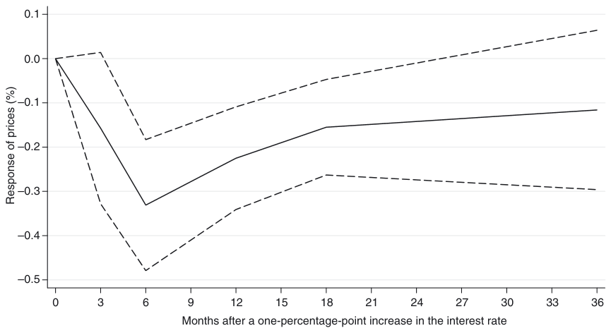
Note: Confidence bands are constructed as +/− one standard error.
We define best practice by selecting methodology characteristics based on the discussion in Section 2: we prefer the output gap over GDP as a measure of economic activity, nonrecursive identification over Cholesky decomposition, data covering a single monetary policy regime over mixing more regimes, and the inclusion of commodity prices and foreign variables instead of omitting them. In addition, we prefer Bayesian estimation since overparameterization can be a problem even for systems of modest size (Banbura, Giannone, and Reichlin 2010). We insert sample maximums for the number of observations, the year of the data, and the number of endogenous variables. Country-specific variables and dummy variables for central bankers and policymakers are set to their sample means. Similar to the previous section, the estimate of the impulse response is corrected for funnel plot asymmetry (i.e., for publication bias or any other bias contributing to the asymmetry, such as small-sample bias).
The estimated impulse response implied by best practice is depicted in Figure 6. After controlling for both publication and misspecification biases, the price puzzle is not present and prices bottom out 6 months after a 1 percentage point increase in the interest rate. The maximum decrease in the price level reaches 0.33% and is statistically significant at the 5% level. The transmission of monetary policy shocks is quick, which contrasts with the view held at many central banks that there are long lags in the effects of monetary policy on prices (e.g., Bank of England 1999, European Central Bank 2010). The absence of the price puzzle is robust both individually and cumulatively to other possible definitions of best practice: selecting the FAVAR approach instead of the Bayesian approach, selecting the specification using sign restrictions instead of nonrecursive identification, or selecting the sample mean of the number of endogenous variables in the VAR system instead of the sample maximum. The price puzzle does not occur even if we set the level of financial development to the sample maximum.
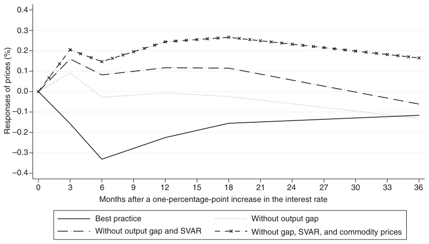
| Implied responses of prices to monetary contraction (in %) | |||||
|---|---|---|---|---|---|
| Horizon | 3 months | 6 months | 12 months | 18 months | 36 months |
| Best practice | −0.157 | −0.331** | −0.225* | −0.155 | −0.116 |
| Without output gap | 0.092 | −0.028 | −0.006 | −0.024 | −0.131 |
| Without gap and SVAR | 0.160** | 0.082 | 0.117 | 0.115 | −0.061 |
| Without gap, SVAR, and commodity prices | 0.205** | 0.147** | 0.244** | 0.266** | 0.165 |
Notes: The values represent the percentage response of prices to a 1 percentage point increase in the interest rate. Without output gap = best practice omitting output gap; Without gap and SVAR = best practice omitting output gap and using recursive identification; Without gap, SVAR, and commodity prices = best practice omitting output gap, using recursive identification, and omitting commodity prices. ** and * denote significance at the 50% and 10% levels, respectively.
To illustrate the consequences of misspecifications for the reported impulse responses, Table 5 and Figure 7 investigate the cases where some aspects of methodology deviate from best practice. When the model does not control for the potential output of the economy, the price puzzle occurs, but prices decline in the medium and long run. When the model combines the omission of the output gap with the use of recursive identification, the puzzle gets stronger and becomes statistically significant, and prices decline below the initial level only after 18 months. When the model additionally omits a measure of commodity prices, the price level is reported never to decline below the initial level during the 3-year horizon after monetary tightening. In sum, our analysis of the VAR studies on monetary transmission indicates that the price puzzle arises systematically from misspecifications of the estimated models.
5. CONCLUSION
We examine the impact of monetary policy shocks on the price level by quantitatively reviewing the impulse response functions from previously published VAR studies on monetary transmission. We collect impulse responses produced by 103 researchers for 31 countries and regress the point estimates on variables capturing study design and country characteristics. To account for within-study dependence in the estimates, we employ mixed-effects multilevel meta-regression. Recently developed meta-analysis methods allow us to estimate the underlying effect of monetary policy implied by the entire literature corrected for potential publication selection and the misspecifications of some VAR models in primary studies.
Our results indicate some evidence of publication selection against the price puzzle, and the selection seems to strengthen for responses with longer horizons after monetary tightening. The finding is in line with Doucouliagos and Stanley (Forthcoming), who suggest that publication selection is likely to be stronger for research areas with less theory competition. Macroeconomists agree about the effects of monetary policy on prices in the long run: prices should eventually decrease after a contraction. On the other hand, a smaller consensus arises regarding the exact effects of monetary policy in the short run because of the cost channel, for example. Published results often exhibit the price puzzle for the short run; on the contrary, results showing the price puzzle for the long run would be difficult to publish.
Next, we find that the reported responses of prices to a monetary tightening are systematically affected by study design and country-specific characteristics. Study design is important in particular for the short-run response. When researchers report the price puzzle, they are likely to omit commodity prices, omit potential output, and use recursive identification in their VAR model. When the biases associated with such misspecifications are filtered out, the impulse response function inferred from the entire literature becomes hump-shaped with no evidence of the price puzzle. The maximum decrease in the price level following a 1 percentage point increase in the interest rate reaches 0.33% and occurs half a year after the tightening.
Finally, our results suggest that the long-run response of prices depends on the characteristics of the examined country; on average, the decrease in prices after a monetary contraction is relatively persistent and does not disappear within three years. The long-run effect of monetary policy is weaker in countries with high average inflation, possibly because high inflation hampers the credibility of the central bank. The effect is stronger in open economies, in countries with a more independent central bank, and during recessions.
For the sake of comparability, in this paper we only include studies using the price level in their VAR models. The robustness of our results could be further examined by conducting a meta-analysis on studies using the inflation rate. In general, the presented method of quantitative synthesis for graphical results can be applied to any other field that uses VARs as a research tool—such as the literature estimating fiscal multipliers.
APPENDIX A: ROBUSTNESS CHECKS
| OLS with clustered standard errors | |||||
|---|---|---|---|---|---|
| Horizon | 3 months | 6 months | 12 months | 18 months | 36 months |
| Intercept (bias) | −0.277 (0.176) | −0.407** (0.186) | −0.341** (0.156) | −0.393** (0.147) | −0.784*** (0.122) |
| 1/SE (effect) | 0.032** (0.014) | 0.033 (0.021) | −0.007 (0.016) | −0.025* (0.014) | −0.018* (0.008) |
| R2 | 0.05 | 0.03 | 0.00 | 0.02 | 0.01 |
| Observations | 208 | 215 | 215 | 217 | 205 |
| Studies | 69 | 70 | 70 | 70 | 63 |
Notes: Standard errors, clustered at the study level, in parentheses. Response variable: the approximated t-statistic of the estimate of the percentage response of prices to a one percentage point increase in the interest rate. ***, **, and * denote significance at the 1%, 5%, and 10% levels, respectively.
| OLS with clustered standard errors | |||||
|---|---|---|---|---|---|
| Horizon | 3 months | 6 months | 12 months | 18 months | 36 months |
| Intercept (bias) | −0.131 (0.151) | −0.127 (0.133) | −0.240* (0.128) | −0.221* (0.120) | −0.538*** (0.130) |
| 1/SE | −0.058 (0.068) | −0.106 (0.115) | −0.237 (0.178) | −0.168 (0.174) | −0.028 (0.212) |
| Structural heterogeneity | |||||
| GDP growth | −0.008 (0.008) | 0.010 (0.010) | 0.024* (0.013) | 0.027* (0.014) | 0.037 (0.024) |
| Inflation | −0.000 (0.004) | −0.003 (0.004) | 0.003 (0.003) | 0.005** (0.002) | 0.008*** (0.002) |
| Inflation volatility | −0.000 (0.001) | 0.001 (0.002) | −0.001 (0.001) | −0.002** (0.001) | −0.003*** (0.001) |
| Financial development | 0.093*** (0.030) | 0.079 (0.054) | 0.174** (0.076) | 0.110 (0.073) | −0.054 (0.067) |
| Openness | −0.026 (0.031) | −0.052 (0.048) | −0.089* (0.048) | −0.130*** (0.048) | −0.258** (0.117) |
| CB independence | 0.038 (0.068) | −0.141 (0.106) | −0.135 (0.133) | −0.258** (0.123) | −0.338*** (0.061) |
| Data characteristics | |||||
| No. of observations | 0.020* (0.011) | 0.043** (0.019) | 0.053** (0.023) | 0.074*** (0.025) | 0.127*** (0.047) |
| Average year | 0.001 (0.001) | −0.001 (0.002) | 0.004 (0.002) | 0.006** (0.002) | 0.012*** (0.003) |
| Specification characteristics | |||||
| GDP deflator | −0.004 (0.013) | 0.023 (0.021) | 0.119*** (0.039) | 0.141*** (0.046) | 0.119* (0.060) |
| Single regime | 0.038** (0.015) | 0.034 (0.022) | 0.024 (0.028) | 0.021 (0.032) | 0.109** (0.053) |
| Commodity prices | −0.047*** (0.008) | −0.070*** (0.018) | −0.139*** (0.023) | −0.158*** (0.027) | −0.212*** (0.059) |
| Foreign variables | 0.009 (0.015) | 0.041*** (0.013) | 0.068** (0.030) | 0.071* (0.038) | 0.082 (0.055) |
| OLS with clustered standard errors | |||||
|---|---|---|---|---|---|
| Horizon | 3 months | 6 months | 12 months | 18 months | 36 months |
| No. of variables | −0.022* (0.012) | −0.024** (0.011) | −0.039** (0.016) | −0.059*** (0.022) | −0.153*** (0.038) |
| Industrial production | 0.024 (0.016) | 0.062*** (0.018) | 0.065** (0.032) | 0.069* (0.040) | −0.026 (0.041) |
| Output gap | −0.259*** (0.090) | −0.330*** (0.102) | −0.235*** (0.060) | −0.140*** (0.039) | 0.012 (0.031) |
| Other measure | −0.094*** (0.022) | −0.066** (0.030) | −0.065 (0.058) | −0.044 (0.077) | 0.018 (0.079) |
| Estimation characteristics | |||||
| BVAR | 0.136*** (0.026) | 0.099*** (0.027) | 0.105* (0.055) | 0.146 (0.089) | 0.131 (0.164) |
| FAVAR | −0.084*** (0.025) | −0.118*** (0.037) | −0.073 (0.054) | 0.029 (0.063) | 0.270*** (0.068) |
| SVAR | −0.089*** (0.018) | −0.142*** (0.026) | −0.139*** (0.031) | −0.147*** (0.030) | −0.050 (0.033) |
| Sign restrictions | −0.300*** (0.031) | −0.299*** (0.042) | −0.347*** (0.061) | −0.396*** (0.096) | −0.250 (0.172) |
| Publication characteristics | |||||
| Central banker | 0.024* (0.014) | 0.058** (0.023) | 0.089** (0.035) | 0.102** (0.040) | 0.125*** (0.036) |
| Policymaker | −0.051** (0.023) | −0.006 (0.022) | 0.070** (0.033) | 0.089*** (0.032) | 0.119*** (0.033) |
| R2 | 0.59 | 0.58 | 0.48 | 0.47 | 0.45 |
| Observations | 208 | 215 | 215 | 217 | 205 |
| Studies | 69 | 70 | 70 | 70 | 63 |
Notes: Standard errors, clustered at the study level, in parentheses. Response variable: the approximated t-statistic of the estimate of the percentage response of prices to a 1 percentage point increase in the interest rate. ***, **, and * denote significance at the 1%, 5%, and 10% levels, respectively.
APPENDIX B: STUDIES USED IN THE META-ANALYSIS
Andries, Marius Alin. (2008) “Monetary Policy Transmission Mechanism in Romania—A VAR Approach.” Theoretical and Applied Economics, 11(528), 250–60.
Anzuini, Alessio, and Aviram Levy. (2007) “Monetary Policy Shocks in the New EU Members: A VAR Approach.” Applied Economics, 39, 1147–61.
Arin, K. Peren, and Sam P. Jolly. (2005) “Trans-Tasman Transmission of Monetary Shocks: Evidence from a VAR Approach.” Atlantic Economic Journal, 33, 267–83.
Bagliano, Fabio C., and Carlo A. Favero. (1998) “Measuring Monetary Policy with VAR Models: An Evaluation.” European Economic Review, 42, 1069–1112.
Bagliano, Fabio C., and Carlo A. Favero. (1999) “Information from Financial Markets and VAR Measures of Monetary Policy.” European Economic Review, 43, 825–37.
Banbura, Marta, Domenico Giannone, and Lucrezia Reichlin. (2010) “Large Bayesian Vector Auto Regressions.” Journal of Applied Econometrics, 25, 71–92.
Belviso, Francesco, and Fabio Milani. (2006) “Structural Factor-Augmented VARs (SFAVARs) and the Effects of Monetary Policy.” B.E. Journal of Macroeconomics: Topics in Macroeconomics, 6, 1–44.
Bernanke, Ben, Jean Boivin, and Piotr S. Eliasz. (2005) “Measuring the Effects of Monetary Policy: A Factor-Augmented Vector Autoregressive (FAVAR) Approach.” Quarterly Journal of Economics, 120, 387–422.
Bernanke, Ben, Mark Gertler, and Mark Watson. (1997) “Systematic Monetary Policy and the Effects of Oil Price Shocks.” Brookings Papers on Economic Activity, 1, 91–142.
Berument, Hakan. (2007) “Measuring Monetary Policy for a Small Open Economy: Turkey.” Journal of Macroeconomics, 29, 411–30.
Boivin, Jean, and Marc P. Giannoni. (2007) “Global Forces and Monetary Policy Effectiveness.” In International Dimensions of Monetary Policy, pp. 429–478. Cambridge, MA: National Bureau of Economic Research, Inc.
Borys, Magdalena, Roman Horvath, and Michal Franta. (2009) “The Effects of Monetary Policy in the Czech Republic: An Empirical Study.” Empirica, 36, 419–43.
Bredin, Don, and Gerard O’Reilly. (2004) “An Analysis of the Transmission Mechanism of Monetary Policy in Ireland.” Applied Economics, 36, 49–58.
Brissimis, Sophocles N., and Nicholas S. Magginas. (2006) “Forward-Looking Information in VAR Models and the Price Puzzle.” Journal of Monetary Economics, 53, 1225–34.
Brunner, Allan D. (2000) “On the Derivation of Monetary Policy Shocks: Should We Throw the VAR Out with the Bath Water?” Journal of Money, Credit, and Banking, 32, 254–79.
Buckle, Robert A., Kunhong Kim, Heather Kirkham, Nathan McLellan, and Jarad Sharma. (2007) “A Structural VAR Business Cycle Model for a Volatile Small Open Economy.” Economic Modelling, 24, 990–1017.
Cespedes, Brisne, Elcyon Lima, and Alexis Maka. (2008) “Monetary Policy, Inflation and the Level of Economic Activity in Brazil after the Real Plan: Stylized Facts from SVAR Models.” Revista Brasileira de Economia, 62, 123–160.
Christiano, Lawrence J., Martin Eichenbaum, and Charles Evans. (1996) “The Effects of Monetary Policy Shocks: Evidence from the Flow of Funds.” Review of Economics and Statistics, 78, 16–34.
Christiano, Lawrence J., Martin Eichenbaum, and Charles L. Evans. (1999) “Monetary Policy Shocks: What Have We Learned and to What End?” In Handbook of Macroeconomics, Vol. 1, edited by J. B. Taylor and M. Woodford, pp. 65–148. Amsterdam, The Netherlands: Elsevier.
Croushore, Dean, and Charles L. Evans. (2006) “Data Revisions and the Identification of Monetary Policy Shocks.” Journal of Monetary Economics, 53, 1135–60.
Cushman, David O. and Tao Zha. (1997) “Identifying Monetary Policy in a Small Open Economy under Flexible Exchange Rates.” Journal of Monetary Economics, 39, 433–48.
De Arcangelis, Guiseppe, and Giorgio Di Giorgio. (2001) “Measuring Monetary Policy Shocks in a Small Open Economy.” Economic Notes, 30, 81–107.
Dedola, Luca, and Francesco Lippi. (2005) “The Monetary Transmission Mechanism: Evidence from the Industries of Five OECD Countries.” European Economic Review, 49, 1543–69.
EFN. (2004) “Monetary Transmission in Acceding Countries.” In European Forecasting Network Annex 53, p. 97142. Florence, Italy: European University Institute.
Eichenbaum, Martin. (1992) “Comment on ‘Interpreting the Macroeconomic Time Series Facts: The Effects of Monetary Policy’.” European Economic Review, 36, 1001–11.
Eickmeier, Sandra, Boris Hofmann, and Andreas Worms. (2009) “Macroeconomic Fluctuations and Bank Lending: Evidence for Germany and the Euro Area.” German Economic Review, 10, 193–223.
Elbourne, Adam. (2008) “The UK Housing Market and the Monetary Policy Transmission Mechanism: An SVAR Approach.” Journal of Housing Economics, 17, 65–87.
Elbourne, Adam, and Jakob de Haan. (2006) “Financial Structure and Monetary Policy Transmission in Transition Countries.” Journal of Comparative Economics, 34, 1–23.
Elbourne, Adam, and Jakob de Haan. (2009) “Modeling Monetary Policy Transmission in Acceding Countries: Vector Autoregression versus Structural Vector Autoregression.” Emerging Markets Finance and Trade, 45, 4–20.
Forni, Mario, and Luca Gambetti. (2010 “The Dynamic Effects of Monetary Policy: A Structural Factor Model Approach.” Journal of Monetary Economics, 57, 203–16.
Fujiwara, Ippei. (2004) “Output Composition of the Monetary Policy Transmission Mechanism in Japan.” Topics in Macroeconomics, 4, 1–21.
Gan, Wee B., and Lee Y. Soon. (2003) “Characterizing the Monetary Transmission Mechanism in a Small Open Economy: The Case of Malaysia.” Singapore Economic Review, 48, 113–34.
Gavin, William T., and David M. Kemme. (2009) “Using Extraneous Information to Analyze Monetary Policy in Transition Economies.” Journal of International Money and Finance, 28, 868–79.
Hanson, Michael S. (2004) “The Price Puzzle Reconsidered.” Journal of Monetary Economics, 51, 1385–1413.
Horvath, Roman, and Marek Rusnak. (2009) “How Important Are Foreign Shocks in a Small Open Economy? The Case of Slovakia.” Global Economy Journal, 9, No. 1.
Hulsewig, Oliver, Eric Mayer, and Timo Wollmershauser. (2006) “Bank Loan Supply and Monetary Policy Transmission in Germany: An Assessment Based on Matching Impulse Responses.” Journal of Banking and Finance, 30, 2893–2910.
Jang, Kyungho, and Masao Ogaki. (2004) “The Effects of Monetary Policy Shocks on Exchange Rates: A Structural Vector Error Correction Model Approach.” Journal of the Japanese and International Economies, 18, 99–114.
Jarocinski, Marek. (2009) “Responses to Monetary Policy Shocks in the East and the West of Europe: A Comparison.” Journal of Applied Econometrics, 25, 833–68.
Jarocinski, Marek, and Frank R. Smets. (2008) “House Prices and the Stance of Monetary Policy.” Federal Reserve Bank of St. Louis Review, 90, 339–65.
Kim, Soyoung. (2001) “International Transmission of U.S. Monetary Policy Shocks: Evidence from VARs.” Journal of Monetary Economics, 48, 339–72.
Kim, Soyoung. (2002) “Exchange Rate Stabilization in the ERM: Identifying European Monetary Policy Reactions.” Journal of International Money and Finance, 21, 413–34.
Krusec, Dejan. (2010) “The Price Puzzle in the Monetary Transmission VARs with Long-Run Restrictions.” Economics Letters, 106, 147–50.
Kubo, Akihiro. (2008) “Macroeconomic Impact of Monetary Policy Shocks: Evidence from Recent Experience in Thailand.” Journal of Asian Economics, 19, 83–91.
Lagana, Gianluca, and Andrew Mountford. (2005) “Measuring Monetary Policy in the UK: A Factor-Augmented Vector Autoregression Model Approach.” Manchester School, 73, 77–98.
Lange, Ronald H. (2010) “Regime-switching Monetary Policy in Canada.” Journal of Macroeconomics, 32, 782–96.
Leeper, Eric M., Christopher A. Sims, and Tao Zha. (1996) “What Does Monetary Policy Do?” Brookings Papers on Economic Activity, 27, 1–78.
Li, Yun Daisy, Talan B. Iscan, and Kuan Xu. (2010) “The Impact of Monetary Policy Shocks on Stock Prices: Evidence from Canada and the United States.” Journal of International Money and Finance, 29, 876–96.
McMillin, W. Douglas. (2001) “The Effects of Monetary Policy Shocks: Comparing Contemporaneous versus Long-Run Identifying Restrictions.” Southern Economic Journal, 67, 618–36.
Mertens, Karel. (2008) “Deposit Rate Ceilings and Monetary Transmission in the US.” Journal of Monetary Economics, 55, 1290–1302.
Minella, Andre. (2003) “Monetary Policy and Inflation in Brazil (1975-2000) A VAR Estimation.” Revista Brasileira de Economia, 57, 605–35.
Mojon, Benoit. (2008) “When Did Unsystematic Monetary Policy Have an Effect on Inflation? European Economic Review, 52, 487–97.
Mojon, Benoit, and Gert Peersman. (2003) “A VAR Description of the Effects of Monetary Policy in the Individual Countries of the Euro Area.” In Monetary Policy Transmission in the Euro Area, edited by A. K. I Angeloni and B. Mojon, pp. 56–74. Cambridge, UK: Cambridge University Press.
Mountford, Andrew. (2005) “Leaning into the Wind: A Structural VAR Investigation of UK Monetary Policy.” Oxford Bulletin of Economics and Statistics, 67, 597–621.
Nakashima, Kiyotaka. (2006) “The Bank of Japan’s Operating Procedures and the Identification of Monetary Policy Shocks: A Reexamination Using the Bernanke-Mihov Approach.” Journal of the Japanese and International Economies, 20, 406–433.
Normandin, Michel, and Louis Phaneuf. (2004) “Monetary Policy Shocks: Testing Identification Conditions under Time-Varying Conditional Volatility.” Journal of Monetary Economics, 51, 1217–43.
Oros, Cornel, and Camelia Romocea-Turcu. (2009) “The Monetary Transmission Mechanisms in the CEECs: A Structural VAR Approach.” Applied Econometrics and International Development, 9, 73–86.
Peersman, Gert. (2004) “The Transmission of Monetary Policy in the Euro Area: Are the Effects Different across Countries? Oxford Bulletin of Economics and Statistics, 66, 285–308.
Peersman, Gert. (2005) “What Caused the Early Millennium Slowdown? Evidence Based on Vector Autoregressions.” Journal of Applied Econometrics, 20, 185–207.
Peersman, Gert, and Frank Smets. (2003) “The Monetary Transmission Mechanism in the Euro Area: More Evidence from VAR Analysis.” In Monetary Policy Transmission on the Euro Area, edited by A. K. I. Angeloni and B. Mojon, pp. 36–55. Cambridge, UK: Cambridge University Press.
Peersman, Gert, and Roland Straub. (2009) “Technology Shocks and Robust Sign Restrictions in a Euro Area SVAR.” International Economic Review, 50, 727–50.
Pobre, Mervin L. (2003) “Sources of Shocks and Monetary Policy in the 1997 Asian Crisis: The Case of Korea and Thailand.” Osaka Economic Papers, 53, 362–73.
Rafiq, M. S., and S. K. Mallick. (2008) “The Effect of Monetary Policy on Output in EMU3: A Sign Restriction Approach.” Journal of Macroeconomics, 30, 1756–91.
Romer, Christina D., and David H. Romer. (2004) “A New Measure of Monetary Shocks: Derivation and Implications.” American Economic Review, 94, 1055–1084.
Shioji, Etsuro. (2000) “Identifying Monetary Policy Shocks in Japan.” Journal of the Japanese and International Economies, 14, 22–42.
Sims, Christopher A., and Tao Zha. (2006) “Were There Regime Switches in U.S. Monetary Policy? American Economic Review, 96, 54–81.
Smets, Frank. (1997) “Measuring Monetary Policy Shocks in France, Germany and Italy: The Role of the Exchange Rate.” Swiss Journal of Economics and Statistics, 133, 597–616.
Sousa, Joao, and Andrea Zaghini. (2008) “Monetary Policy Shocks in the Euro Area and Global Liquidity Spillovers.” International Journal of Finance and Economics, 13, 205–18.
Vargas-Silva, Carlos. (2008) “Monetary Policy and the US Housing Market: A VAR Analysis Imposing Sign Restrictions.” Journal of Macroeconomics, 30, 977–90.
Voss, G. and L. B. Willard. (2009) “Monetary Policy and the Exchange Rate: Evidence from a Two-Country Model.” Journal of Macroeconomics, 31, 708–20.
Wu, Tao. (2003) “Stylized Facts on Nominal Term Structure and Business Cycles: An Empirical VAR Study.” Applied Economics, 35, 901–06.
LITERATURE CITED
Abreu, Maria, Henri L. F. de Groot, and Raymond J. G. M. Florax. (2005) “A Meta-Analysis of β-Convergence: the Legendary 2%.” Journal of Economic Surveys, 19, 389–420.
Angeloni, Ignazio, Luc Aucremanne, Michael Ehrmann, Jordi Galí, Andrew Levin, and Frank Smets. (2006) “New Evidence on Inflation Persistence and Price Stickiness in the Euro Area: Implications for Macro Modeling.” Journal of the European Economic Association, 4, 562–74.
Arnone, Marco, Bernard J. Laurens, Jean-Francois Segalotto, and Martin Sommer. (2009) “Central Bank Autonomy: Lessons from Global Trends.” IMF Staff Papers, 56, 263–296.
Ashenfelter, Orley, and Michael Greenstone. (2004) “Estimating the Value of a Statistical Life: The Importance of Omitted Variables and Publication Bias.” American Economic Review, 94, 454–60.
Banbura, Marta, Domenico Giannone, and Lucrezia Reichlin. (2010) “Large Bayesian Vector Auto Regressions.” Journal of Applied Econometrics, 25, 71–92.
Bank of England. (1999) “The Transmission Mechanism of Monetary Policy. A Paper by the Monetary Policy Committee.” Bank of England, April 1999.
Barth, Marvin J., and Valerie A. Ramey. (2002) “The Cost Channel of Monetary Transmission.” In NBER Macroeconomics Annual 2001, Vol. 16, pp. 199–256. Cambridge, MA: National Bureau of Economic Research.
Bernanke, Ben, Jean Boivin, and Piotr S. Eliasz. (2005) “Measuring the Effects of Monetary Policy: A Factor-augmented Vector Autoregressive (FAVAR) Approach.” Quarterly Journal of Economics, 120, 387–422.
Bernanke, Ben, and Mark Gertler. (1989) “Agency Costs, Net Worth, and Business Fluctuations.” American Economic Review, 79, 14–31.
Bernanke, Ben S. (1986) “Alternative Explanations of the Money-Income Correlation.” Carnegie-Rochester Conference Series on Public Policy, 25, 49–99.
Bernanke, Ben S., and Alan S. Blinder. (1992) “The Federal Funds Rate and the Channels of Monetary Transmission.” American Economic Review, 82, 901–21.
Bernanke, Ben S., and Mark Gertler. (1995) “Inside the Black Box: The Credit Channel of Monetary Policy Transmission.” Journal of Economic Perspectives, 9, 27–48.
Blanchard, Olivier J., and Mark W. Watson. (1986) “Are Business Cycles All Alike?” In The American Business Cycle: Continuity and Change, pp. 123–180. Cambridge, MA: National Bureau of Economic Research.
Boivin, Jean, and Marc P. Giannoni. (2006) “Has Monetary Policy Become More Effective?” Review of Economics and Statistics, 88, 445–62.
Borys, Magdalena, Roman Horvath, and Michal Franta. (2009) “The Effects of Monetary Policy in the Czech Republic: An Empirical Study.” Empirica, 36, 419–43.
Canova, Fabio, and Gianni D. Nicolo. (2002) “Monetary Disturbances Matter for Business Fluctuations in the G-7.” Journal of Monetary Economics, 49, 1131–59.
Card, David, Jochen Kluve, and Andrea Weber. (2010) “Active Labor Market Policy Evaluations: A Meta-analysis.” The Economic Journal, 120, F452–F477.
Card, David, and Alan B. Krueger. (1995) “Time-Series Minimum-Wage Studies: A Meta-analysis.” American Economic Review, 85, 238–43.
Carlstrom, Charles T., Timothy S. Fuerst, and Matthias Paustian. (2009) “Monetary Policy Shocks, Choleski Identification, and DNK Models.” Journal of Monetary Economics, 56, 1014–21.
Cecchetti, Stephen G. (1999) “Legal Structure, Financial Structure, and the Monetary Policy Transmission Mechanism.” Federal Reserve Bank of New York Economic Policy Review, 5, 9–28.
Chetty, Raj, Adam Guren, Day Manoli, and Andrea Weber. (2011) “Are Micro and Macro Labor Supply Elasticities Consistent? A Review of Evidence on the Intensive and Extensive Margins.” American Economic Review, 101, 471–75.
Christiano, Lawrence J., Martin Eichenbaum, and Charles L. Evans. (1999) “Monetary Policy Shocks: What Have We Learned and to What End?” In Handbook of Macroeconomics, edited by J. B. Taylor and M. Woodford, Vol. 1, pp. 65–148. Amsterdam, The Netherlands: Elsevier.
de Grauwe, Paul, and Cláudia C. Storti. (2004) “The Effects of Monetary Policy: A Meta-Analysis.” CESifo Working Paper Series 1224, CESifo Group Munich.
DeLong, J. Bradford, and Kevin Lang. (1992) “Are All Economic Hypotheses False?” Journal of Political Economy, 100, 1257–72.
Dennis, Richard, Kai Leitemo, and Ulf Söderström. (2007) “Monetary Policy in a Small Open Economy with a Preference for Robustness.” Working Paper Series 2007-04, Federal Reserve Bank of San Francisco.
Disdier, Anne-Célia, and Keith Head. (2008) “The Puzzling Persistence of the Distance Effect on Bilateral Trade.” Review of Economics and Statistics, 90, 37–48.
Doucouliagos, Hristos, and T. D. Stanley. (2009) “Publication Selection Bias in Minimum-Wage Research? A Meta-Regression Analysis.” British Journal of Industrial Relations, 47, 406–28.
Doucouliagos, Hristos, and T. D. Stanley. (Forthcoming) “Are All Economic Facts Greatly Exaggerated? Theory Competition and Selectivity.” Journal of Economic Surveys.
Egert, Balázs, and Ronald MacDonald. (2009) “Monetary Transmission Mechanism in Central and Eastern Europe: Surveying the Surveyable.” Journal of Economic Surveys, 23(2), 277–327.
Elbourne, Adam, and Jakob de Haan. (2006) “Financial Structure and Monetary Policy Transmission in Transition Countries.” Journal of Comparative Economics 34(1), 1–23.
European Central Bank. (2010) “Monthly Bulletin.” European Central Bank, May.
Giordani, Paolo. (2004) “An Alternative Explanation of the Price Puzzle.” Journal of Monetary Economics, 51, 1271–96.
Görg, Holger, and Eric Strobl. (2001) “Multinational Companies and Productivity Spillovers: A Meta-analysis.” The Economic Journal, 111, F723–F739.
Hanson, Michael S. (2004) “The Price Puzzle Reconsidered.” Journal of Monetary Economics, 51, 1385–1413.
Havranek, Tomas, and Zuzana Irsova. (2011) “Estimating Vertical Spillovers from FDI: Why Results Vary and What the True Effect Is.” Journal of International Economics, 85, 234–44.
Keefer, Philip, and David Stasavage. (2003) “The Limits to Delegation: Veto Players, Central Bank Independence, and the Credibility of Monetary Policy.” American Political Science Review, 97, 407–23.
Kim, Soyoung, and Nouriel Roubini. (2000) “Exchange Rate Anomalies in the Industrial Countries: A Solution with a Structural VAR Approach.” Journal of Monetary Economics, 45, 561–86.
Krusec, D. (2010) “The Price Puzzle in the Monetary Transmission VARs with Long-Run Restrictions.” Economics Letters, 106, 147–50.
Mohanty, Madhusudan S., and Philip Turner. (2008) “Monetary Policy Transmission in Emerging Market Economies: What Is New?” In Transmission Mechanisms for Monetary Policy in Emerging Market Economies, Vol. 35, pp. 1–59. Basel, Switzerland: Bank for International Settlements.
Nelson, Jon, and Peter Kennedy. (2009) “The Use (and Abuse) of Meta-Analysis in Environmental and Natural Resource Economics: An Assessment.” Environmental and Resource Economics, 42, 345–77.
Perino, Grischa. (2010) “How Delegation Improves Commitment.” Economics Letters, 106, 137–39.
Rabanal, Pau. (2007) “Does Inflation Increase After a Monetary Policy Tightening? Answers Based on an Estimated DSGE Model.” Journal of Economic Dynamics and Control, 31, 906–37.
Rogoff, Kenneth. (1985) “The Optimal Degree of Commitment to an Intermediate Monetary Target.” Quarterly Journal of Economics, 100, 1169–89.
Rose, Andrew K., and Tom D. Stanley. (2005) “A Meta-Analysis of the Effect of Common Currencies on International Trade.” Journal of Economic Surveys, 19, 347–65.
Sims, Christopher A. (1980) “Macroeconomics and Reality.” Econometrica, 48, 1–48.
Sims, Christopher A. (1992) “Interpreting the Macroeconomic Time Series Facts: The Effects of Monetary Policy.” European Economic Review, 36, 975–1000.
Sims, Christopher A., and Tao Zha. (1998) “Bayesian Methods for Dynamic Multivariate Models.” International Economic Review, 39, 949–68.
Sims, Christopher A., and Tao Zha. (1999) “Error Bands for Impulse Responses.” Econometrica, 67, 1113–56.
Slavin, Robert E. (1986) “Best-Evidence Synthesis: An Alternative to Meta-Analytic and Traditional Reviews.” Educational Researcher, 15, 5–11.
Smith, V. Kerry, and Ju-Chin Huang. (1995) “Can Markets Value Air Quality? A Meta-analysis of Hedonic Property Value Models.” Journal of Political Economy, 103, 209–27.
Stanley, Tom D. (2001) “Wheat from Chaff: Meta-Analysis as Quantitative Literature Review.” Journal of Economic Perspectives, 15, 131–50.
Stanley, Tom D. (2004) “Does Unemployment Hysteresis Falsify the Natural Rate Hypothesis? A Meta-Regression Analysis.” Journal of Economic Surveys, 18, 589–612.
Stanley, Tom D. (2008) “Meta-Regression Methods for Detecting and Estimating Empirical Effects in the Presence of Publication Selection.” Oxford Bulletin of Economics and Statistics, 70, 103–27.
Stanley, Tom D., and Hristos Doucouliagos. (2010) “Picture This: A Simple Graph that Reveals Much Ado about Research.” Journal of Economic Surveys, 24, 170–91.
Stock, James H., and Mark W. Watson. (2001) “Vector Autoregressions.” Journal of Economic Perspectives, 15, 101–15.
Uhlig, Harald. (2005) “What Are the Effects of Monetary Policy on Output? Results from an Agnostic Identification Procedure.” Journal of Monetary Economics, 52, 381–419.
Uhlig, Harald. (2010) “Economics and Reality.” NBER Working Papers 16416.
ENDNOTES
- To our knowledge, there has been one unpublished meta-analysis on the impact of monetary policy on prices (de Grauwe and Storti 2004) and it focused solely on heterogeneity in the reported estimates; that is, it did not filter out publication bias and misspecifications to estimate the underlying impulse response.
- Uhlig (2010, p. 17) writes: “At a Carnegie-Rochester conference a few years back, Ben Bernanke presented an empirical paper, in which the conclusions nicely lined up with a priori reasoning about monetary policy. Christopher Sims then asked him, whether he would have presented the results, had they turned out to be at odds instead. His half-joking reply was, that he presumably would not have been invited if that had been so. There indeed is the danger (or is it a valuable principle?) that a priori economic theoretical biases filter the empirical evidence that can be brought to the table in the first place.”
- Additionally, the asymmetry of funnel plots may partly reflect small-sample bias in the estimated VAR coefficients. A similar limitation was found in a meta-analysis of unemployment hysteresis (Stanley 2004).
- We experimented with several nested mixed-effects models, but they yield qualitatively similar outcomes. Additionally, we collected data from unpublished manuscripts appearing in the working paper series of NBER, OECD, IMF, European Commission, and all central banks listed in the Bank for International Settlements Central Bank Research Hub, and ran regression (5) using this new sample. The working papers show a pattern of publication bias very similar to that presented in Table 2. These robustness checks are available in the online appendix.