Lecture 1: Introduction to Meta-Analysis

Meta important for research, policy, practice

Research experience:

• Professor at Charles University, Prague
• Affiliate at the Meta-Research Innovation Center, Stanford
• Panel member at ERC (European Research Council) Advanced

Policy experience:

• Former Advisor to the Board, Czech National Bank
• Former member of the Czech National Economic Council
• Affiliate at the Centre for Economic Policy Research, London

tomashavranek.cz

What happens if the government spends more?

Labor supply elasticity is key (but how to calibrate it?):

Meta in monetary policy making: DSGE models

DSGE = dynamic stochastic general equilibrium

1. The dominant policy analysis and forecasting tool
2. Used by central banks and ministries of finance
3. Micro-based with “deep” parameters
4. Immune to Lucas critique (?)
5. Discipline over intuition
6. Hard to understand for policy makers

Dozens or hundreds of equations

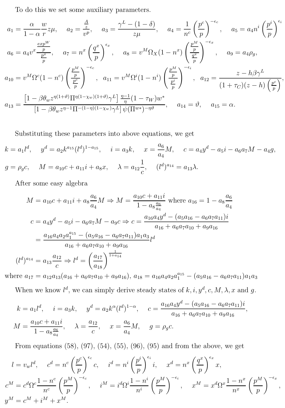
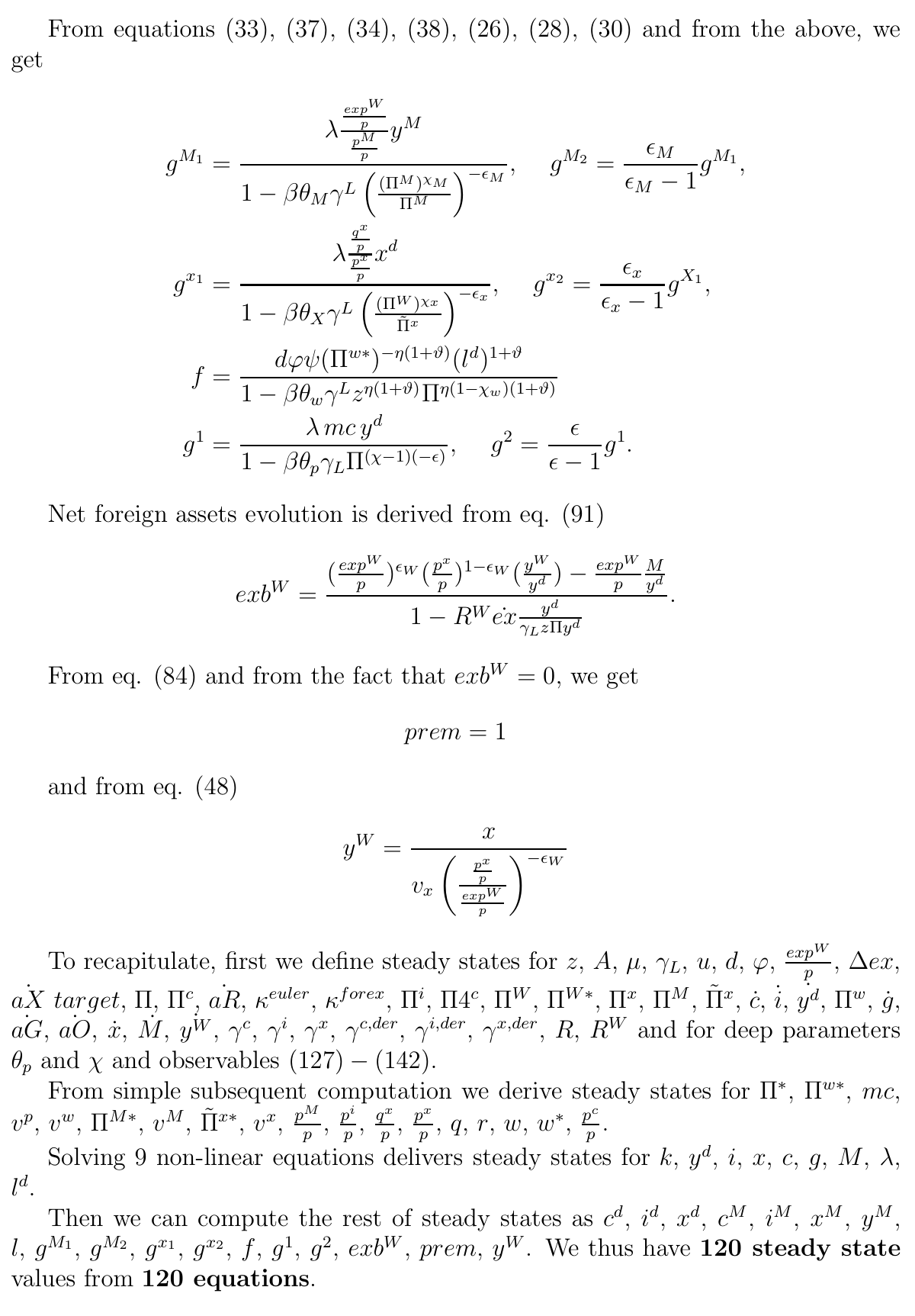
Psychohistory accomplished? Civ VII?

Main output: fan charts

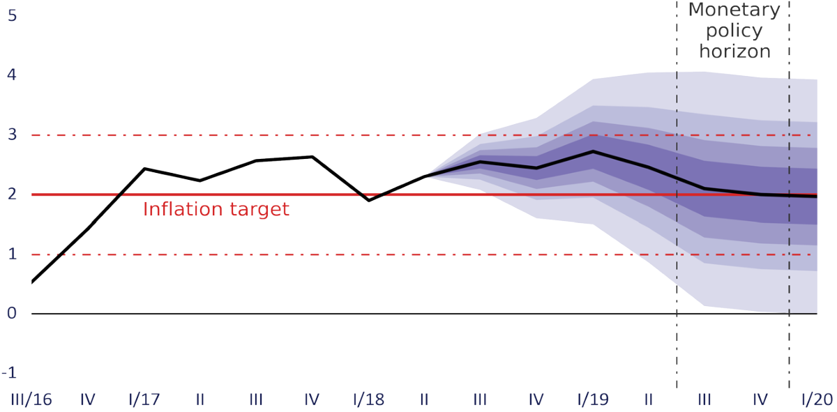
Calibration uncertainty: meta needed!

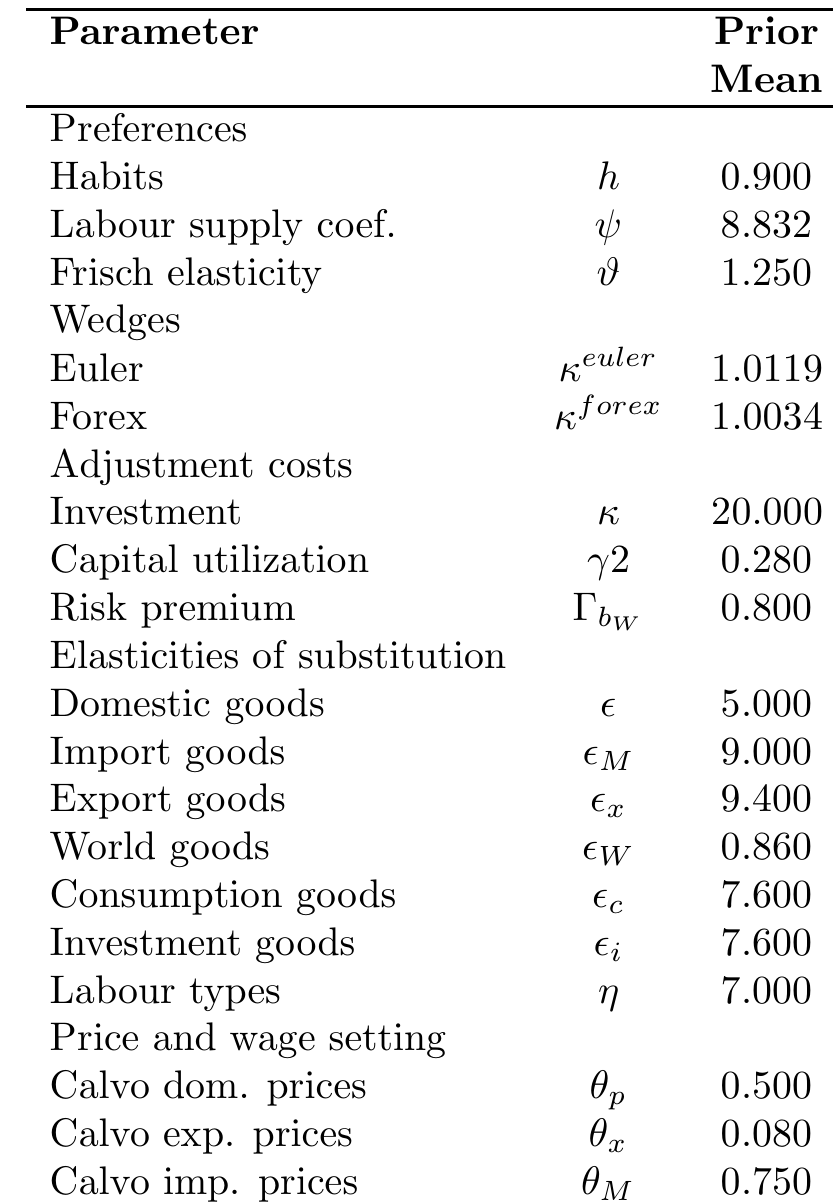
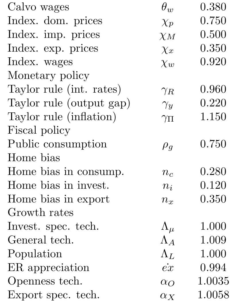
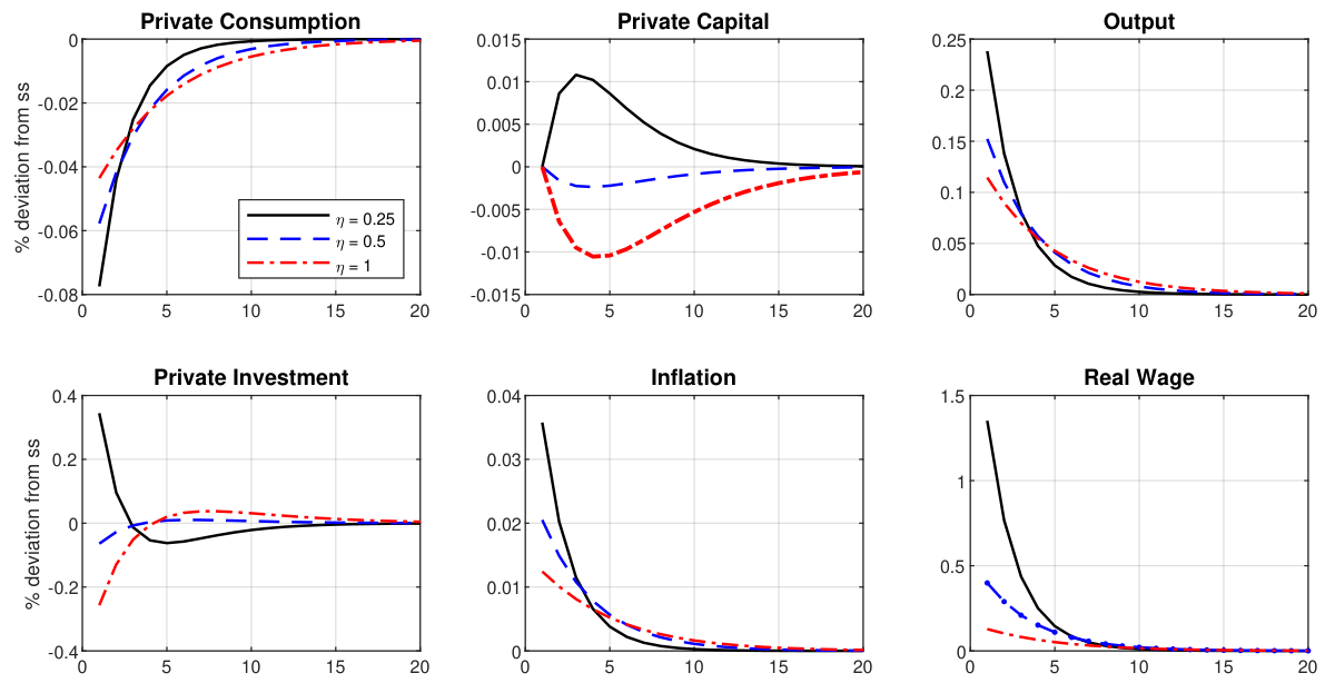
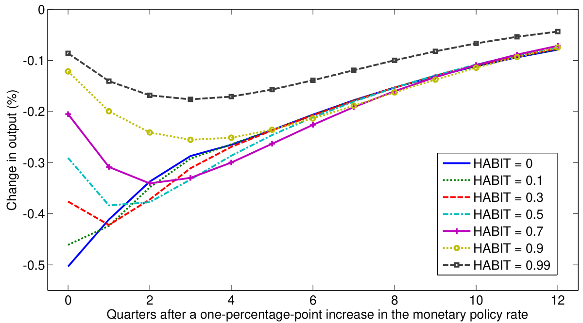
What happens if we change one parameter?

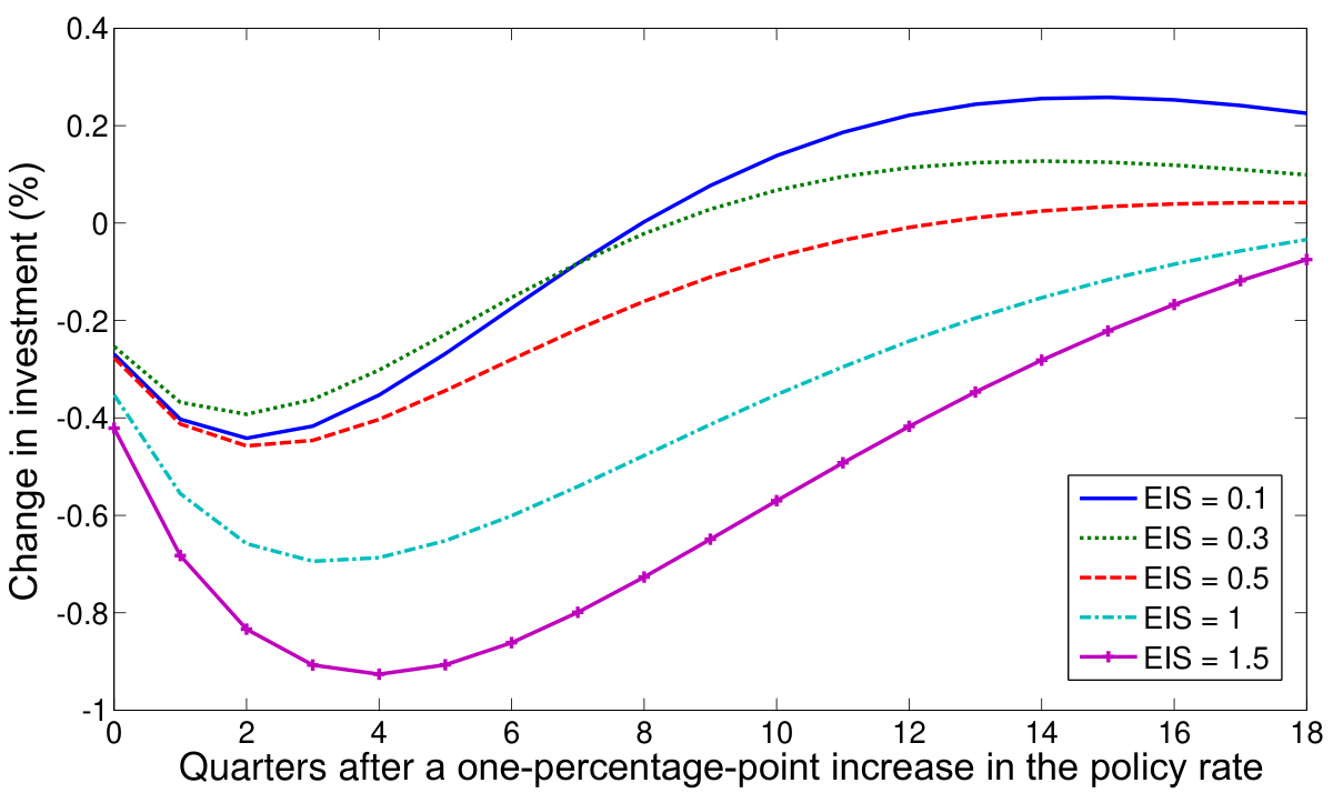
Coincidence? Hardly. Meta-analysis essential

Estimates of the labor supply elasticity vary

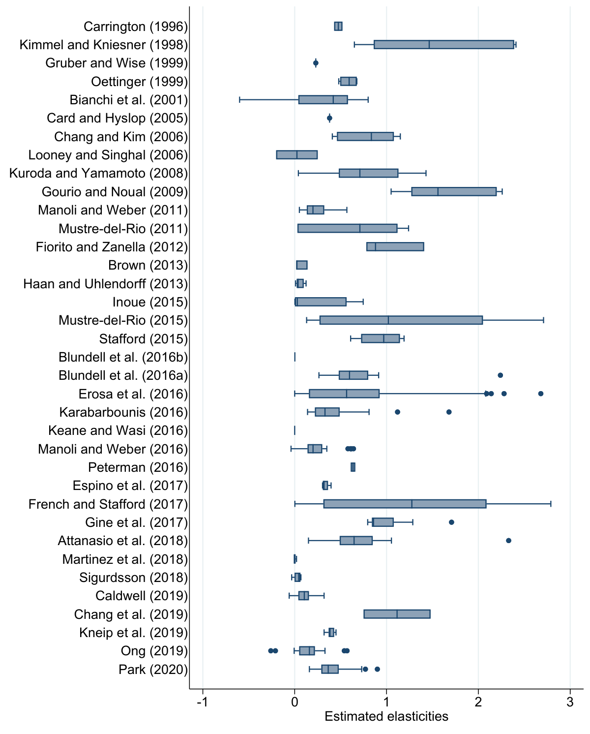
Values around 0.4 to 0.5 used for calibration (CBO)

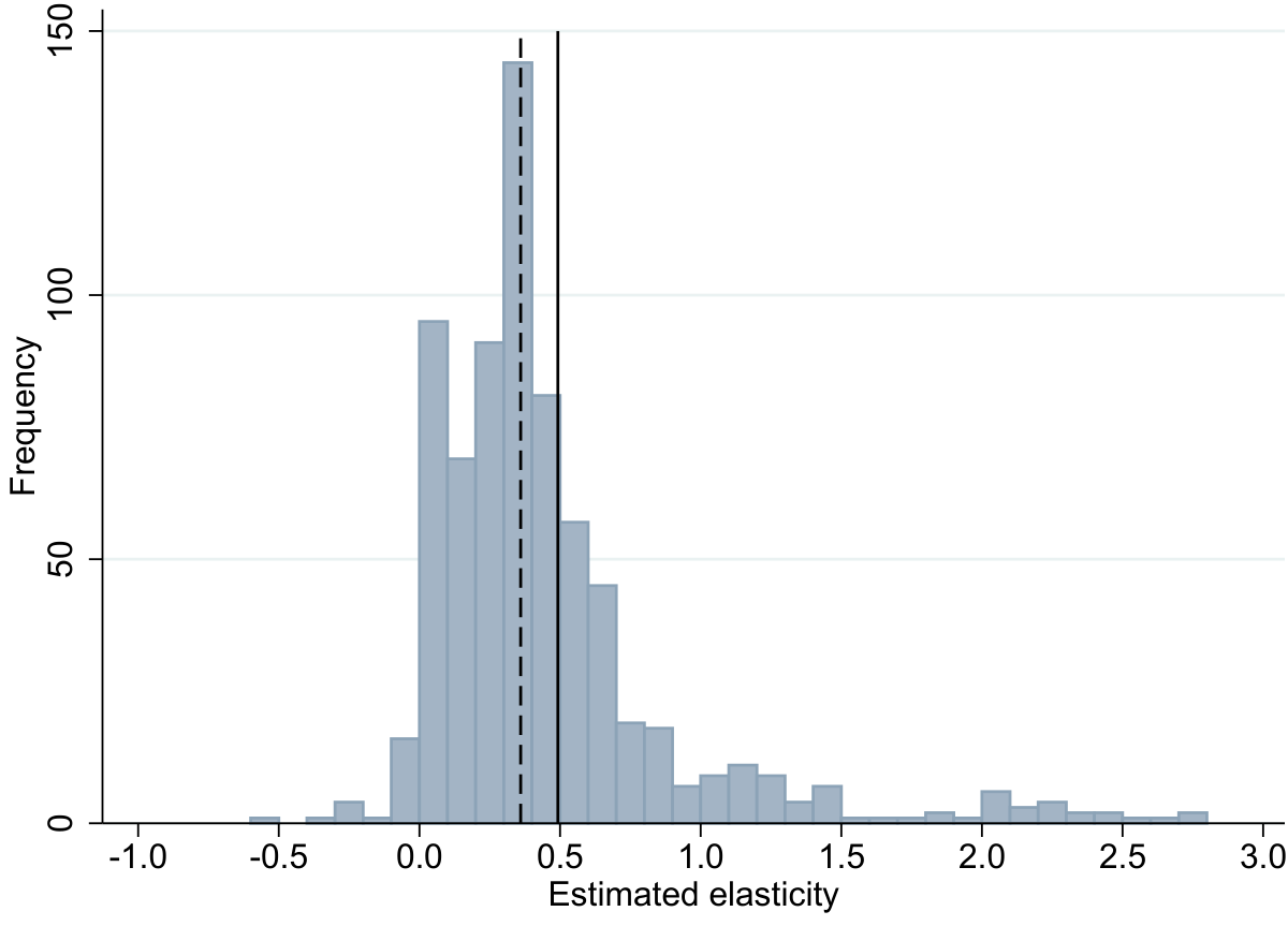
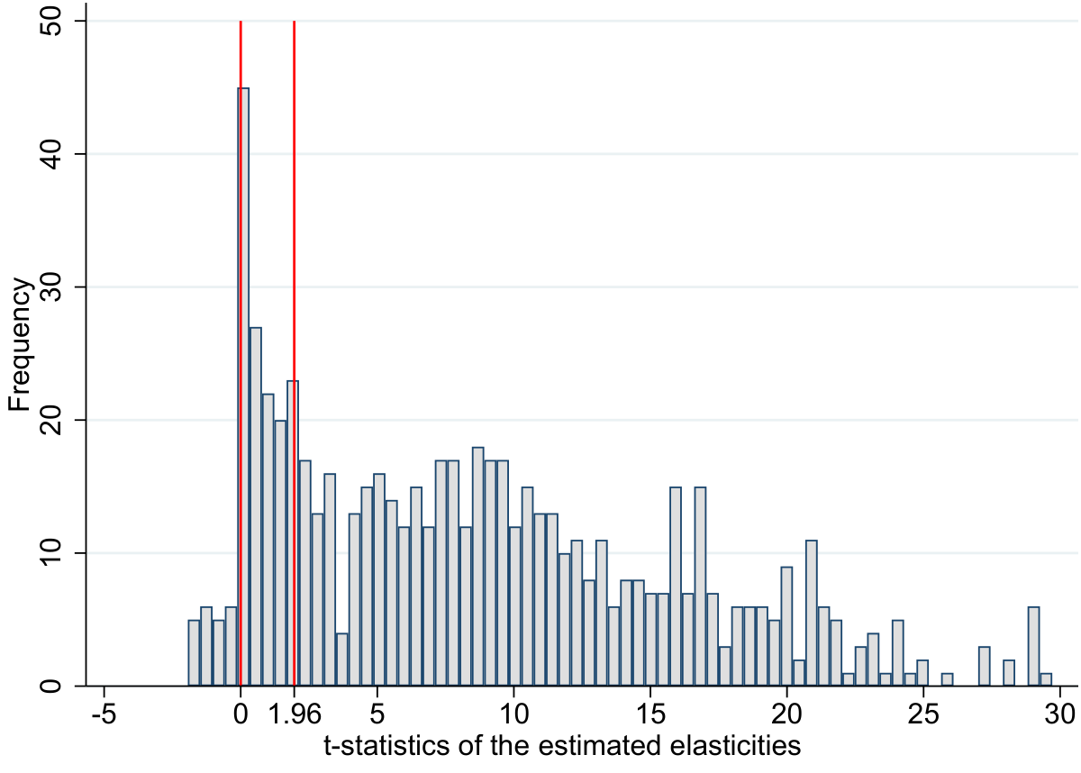
Bias: some estimates less likely to be published

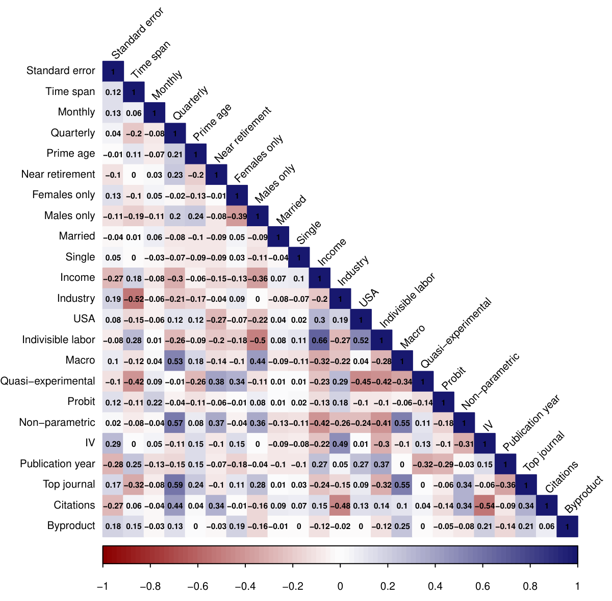
Context: different situations yield different estimates

Implied elasticity: taking bias and context into account

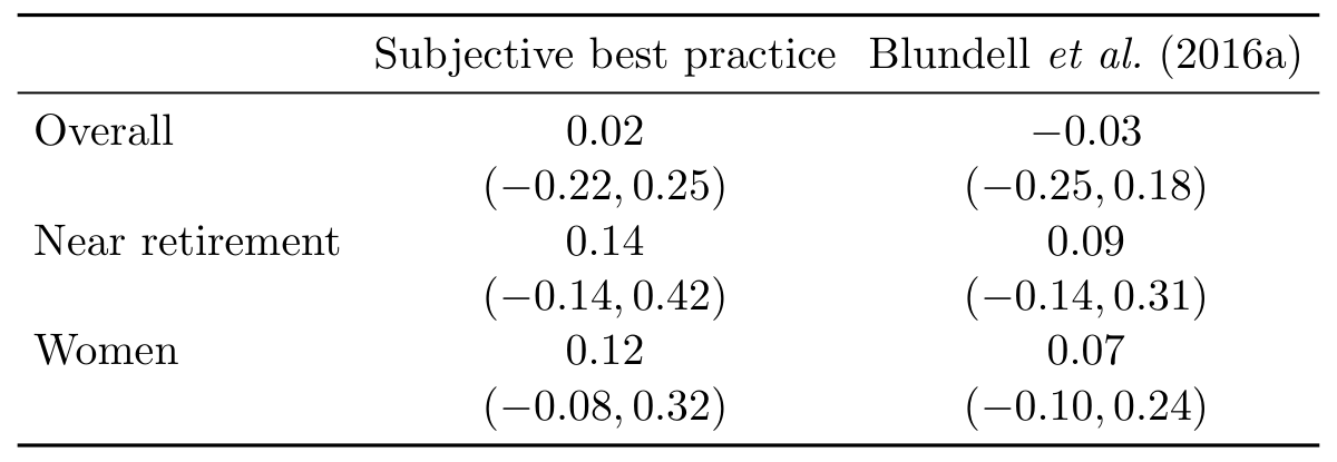
Let's construct a hypothetical study that uses all information reported in the literature but puts more weight on selected aspects (high precision, quasi-experimental setup, etc.)

Course

1. Intro
2. Applied examples
3. Literature search
4. Data collection
5. Basic meta models
6. Replications (student presentations)
7. Publication bias
8. P-hacking
9. Heterogeneity
10. Meta-research
11. Limitations
12. Applications (student presentations)

Grading

• Applied meta-analysis (40%)
• Replication (20%)
• Discussion (20%)
• Activity (10%)
• Attendance (10%)

Guidelines

Resources

meta-analysis.cz

Lecture 2: Applied Meta-Analysis Examples

Example 1: Daylight saving time

When using econometric analysis, researchers typically estimate the following model: ln Consumption_t = α + DST· Treatment effect_t + Controls_t + ε.

• Consumption: the average energy consumption during time t for a given hour, day, and year.
• Treatment effect: equals 1 for all hours when daylight saving time applies.
• Controls: seasonality and holidays, weather, the intensity of sunlight, heterogeneity among consumption units, etc.

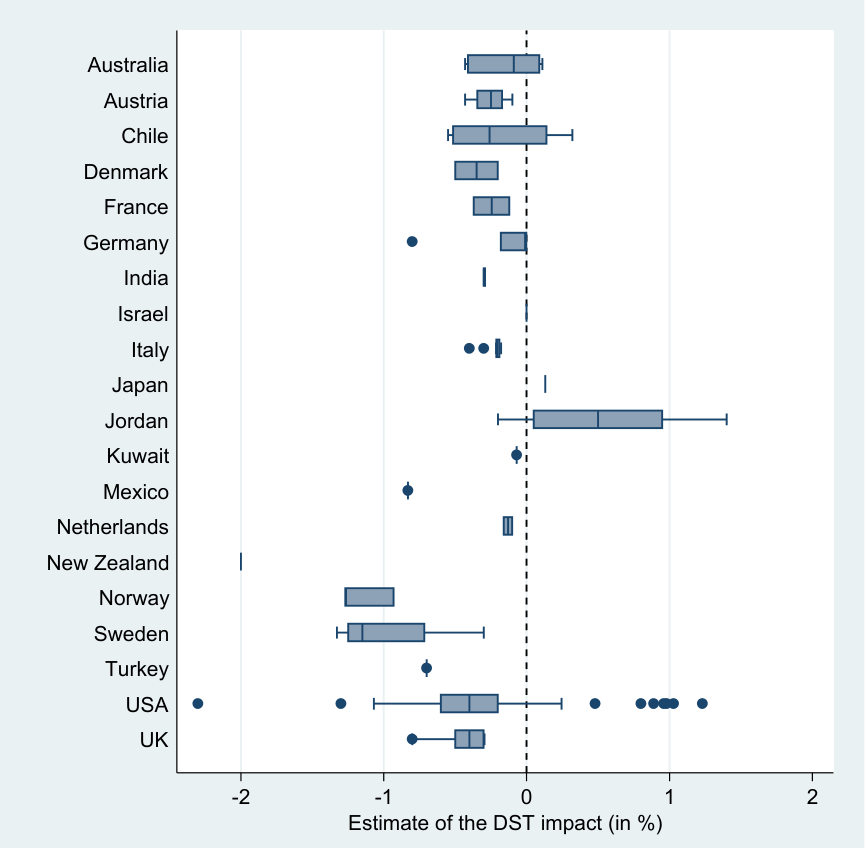
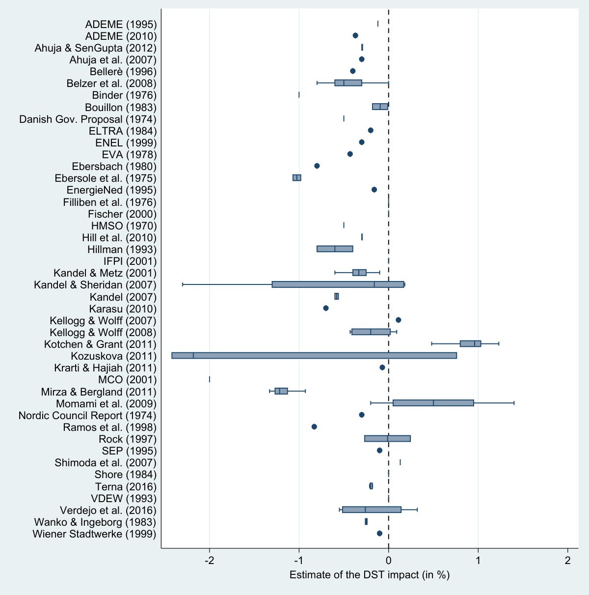
No consensus in the literature

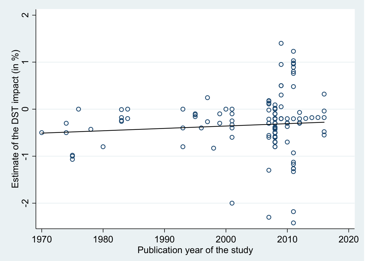
Journals report smaller savings

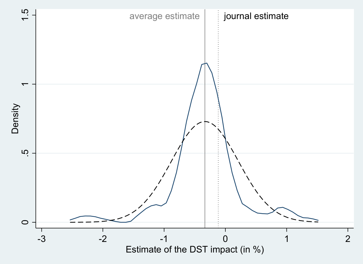
Publication bias? Probably not

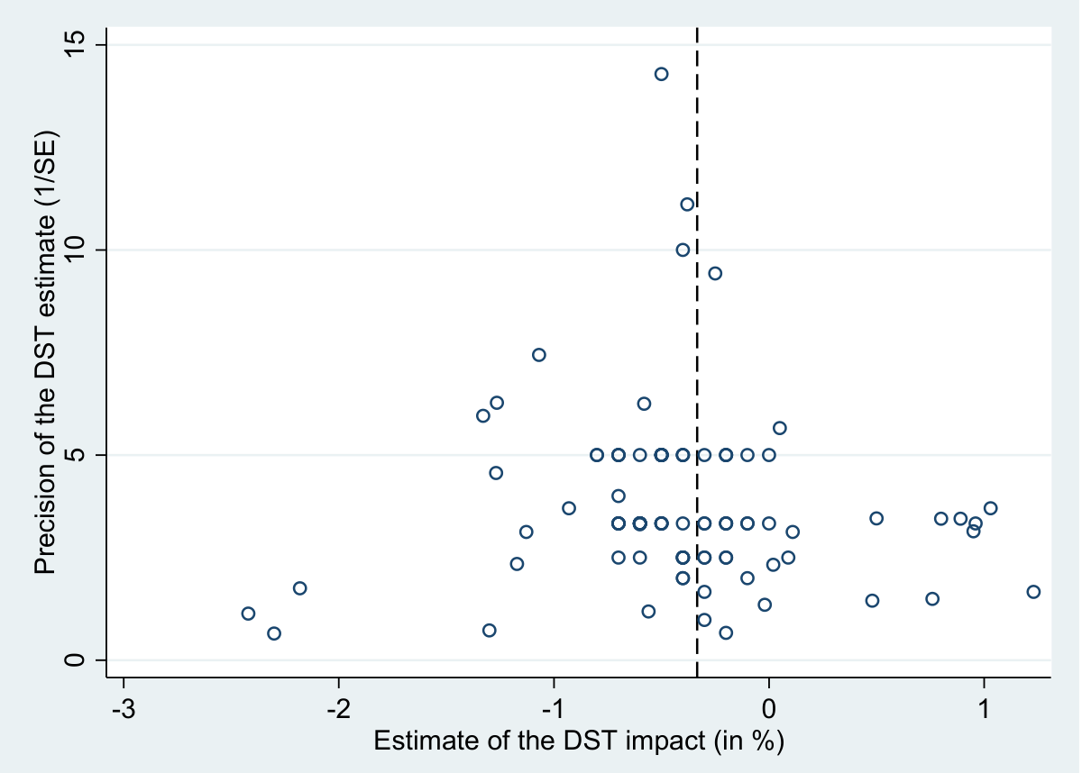
Funnel asymmetry tests

If the ratio of the point estimate to its standard error has a t-distribution, then the two quantities should be independent: estimate_i = β [true effect] + β_0 SE_i [publication bias] + μ_i.

The no. of obs. can be used as an instrument for SE.

 | OLS | FE | BE | Country | ME | IV
SE (publication bias) | -0.410 | -1.217 | -0.410 | -0.496 | -0.449 | 0.226
 | (0.265) | (0.790) | (0.757) | (0.805) | (0.688) | (1.088)
Constant (true effect) | -0.293 *** | -0.222 *** | -0.294 *** | -0.278 *** | -0.291 *** | -0.445 *
 | (0.000778) | (0.0700) | (0.00812) | (0.0459) | (0.00731) | (0.243)
Observations | 101 | 101 | 101 | 101 | 101 | 90

Country heterogeneity

Method heterogeneity (just studies for the US)

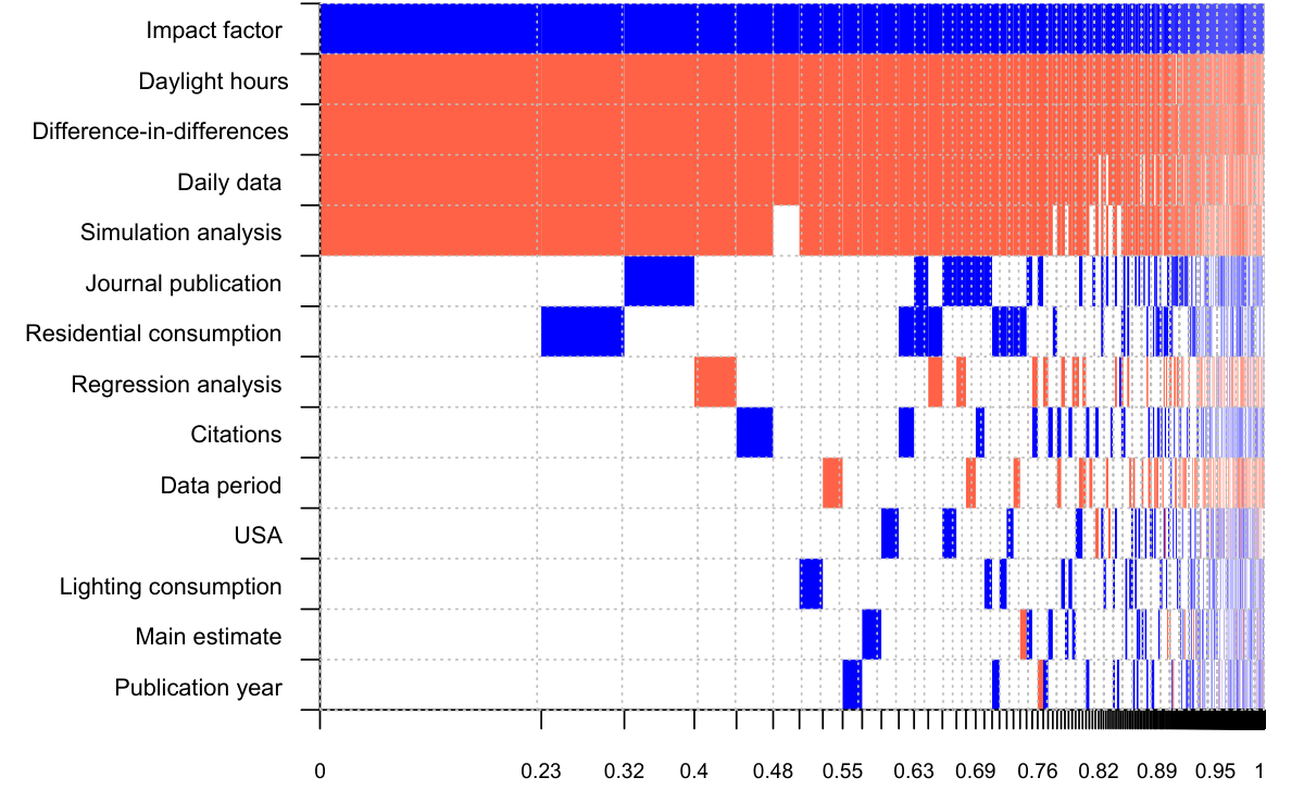
What explains the differences in conclusions? (1)

Data characteristics
Data period | The number of years used in the estimation.
Main estimate | = 1 if the estimate is preferred by the authors of the study.
Hourly data | = 1 if the data are examined on hourly or higher than hourly granularity.
Daily data | = 1 if the data are examined on a daily basis.
Daylight hours | Average time between sunrise and sunset on the longest day for the country or region under examination.
Europe | = 1 if European countries are examined.
USA | = 1 if US data are examined.
Design of the analysis
Regression analysis | = 1 if the primary study is based on regression analysis.
Simulation analysis | = 1 if the study is based on simulation.
Difference-in-diff. | = 1 if the difference-in-differences approach is employed.
Residential cons. | = 1 if only residential consumption is examined.
Lighting cons. | = 1 if total energy savings are reported as a result of lighting reduction.

What explains the differences in conclusions? (2)

Publication characteristics
Publication year | The publication year of the study (base = 1970).
Journal article | = 1 if the study was published in a peer-reviewed journal.
Impact factor | The recursive RePEc impact factor of the outlet.
Citations | The logarithm of the total number of citations of the study in Google Scholar.

Bayesian model averaging

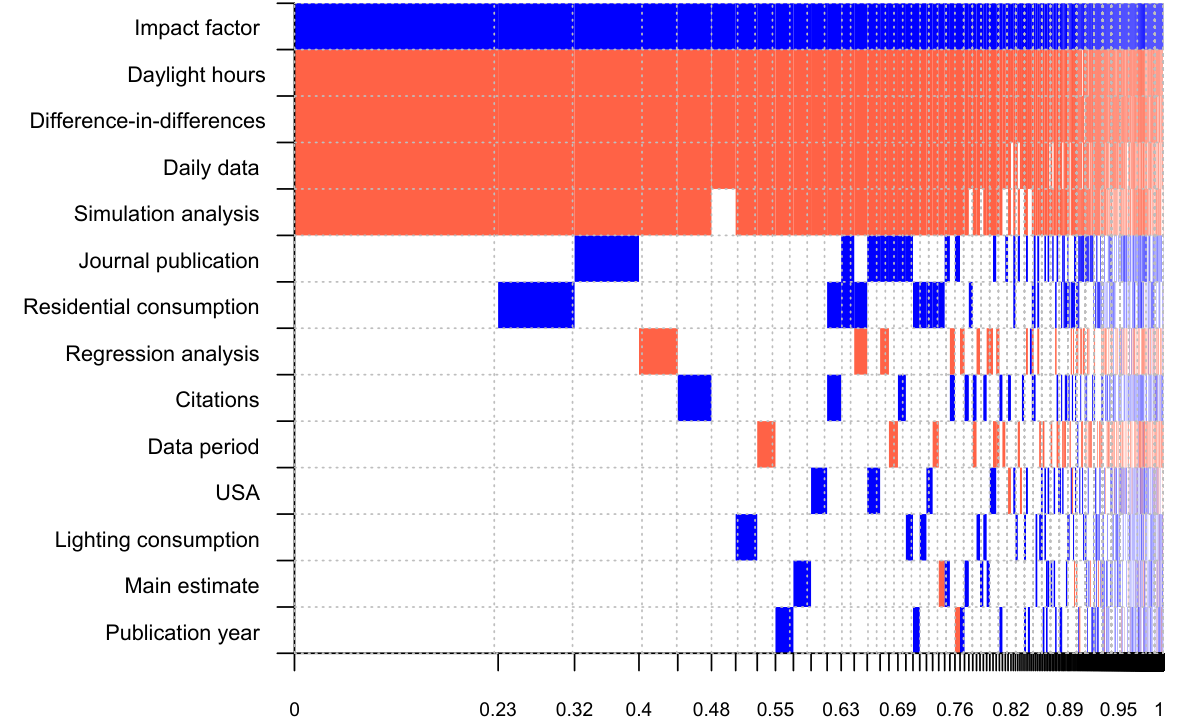
Results

1. The mean reported estimate suggests energy savings of 0.34% due to DST.
2. The results are driven by the method employed (simulation vs. regression).
3. Energy savings are larger for countries farther away from the equator.

www.meta-analysis.cz/dst

For further reading

• Stanley, T. D. & C. Doucouliagos (2012): Meta-Regression Analysis in Economics and Business. Routledge, 1st. edition.
• Brodeur, A., M. Sangnier & Y. Zylberg (2016): Star Wars: The Empirics Strike Back. AEJ Applied 8(1): pp. 1 to 32.
• Havranek, T. (2015): Measuring Intertemporal Substitution: The Importance of Method Choices and Publication Bias. JEEA 13(6): pp. 1180 to 1204.

Reading list on RePEc: Google “meta-analysis in economics.”

Example 2: Interest rates and house prices

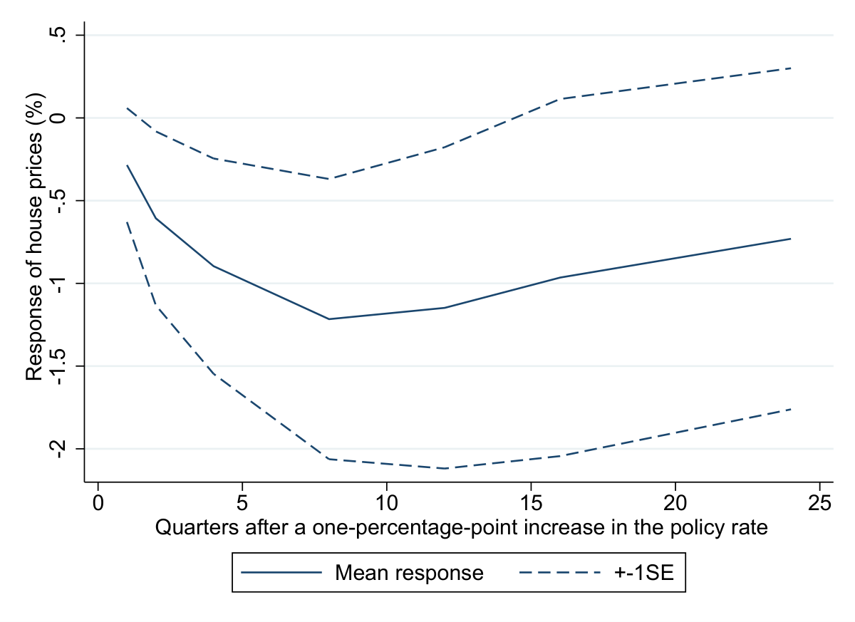
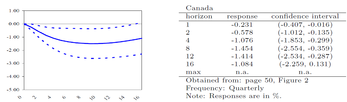
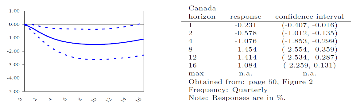
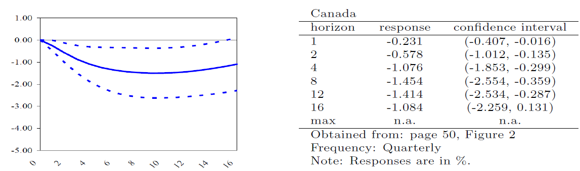
Converting graphs to data

We measure pixel coordinates using WebPlotDigitizer:

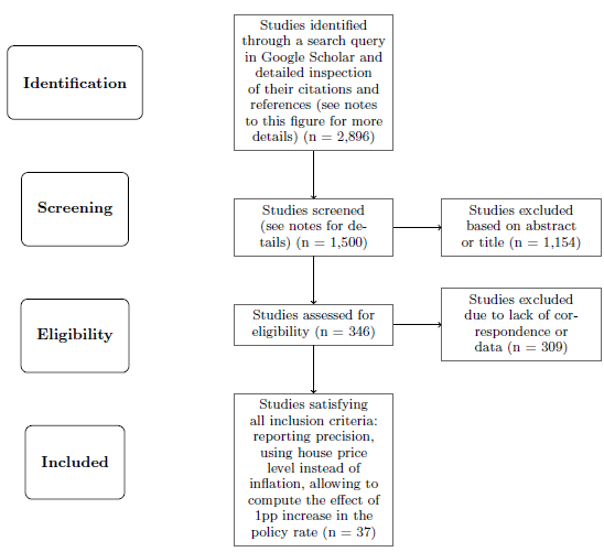
Literature search

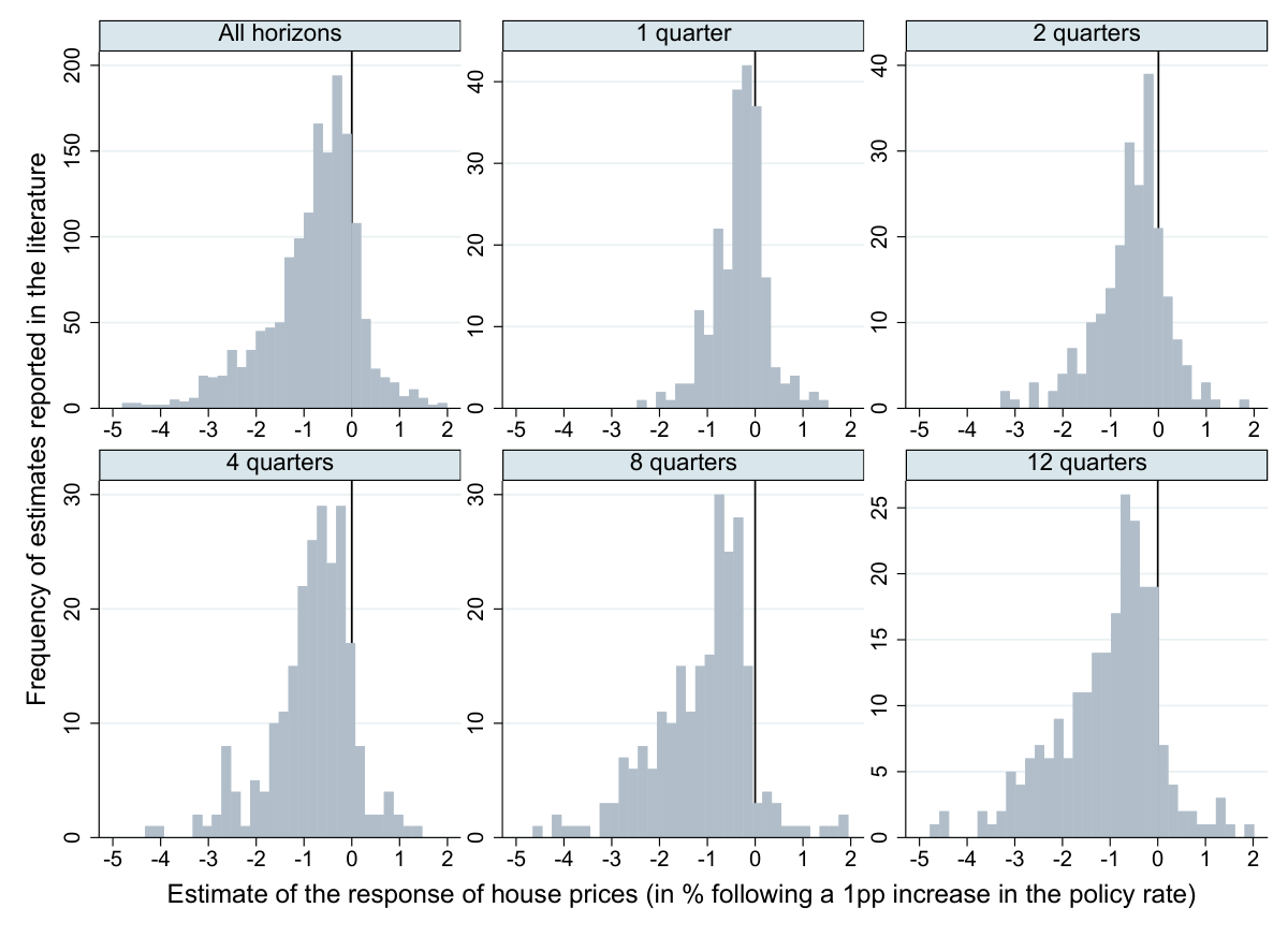
Histograms for different horizons

Funnel asymmetry test (Card & Krueger)

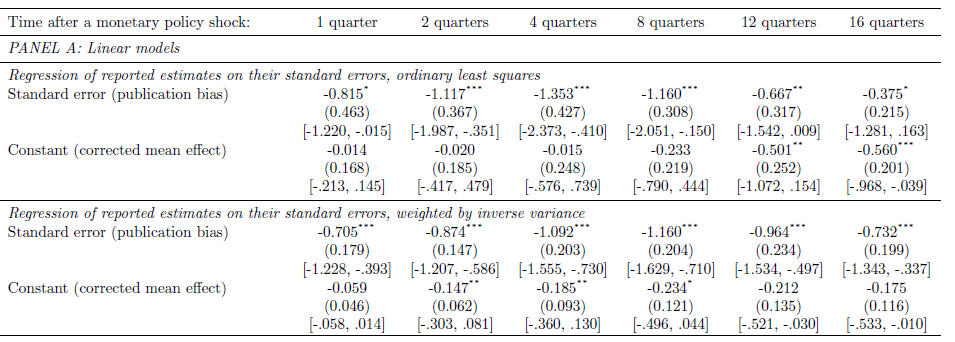
In the absence of publication bias the funnel should be symmetrical: estimate_i = β [true effect] + β_0 SE_i [publication bias] + μ_i.

The equation is heteroscedastic. Weighted least squares yield

t_i = β_0 + β (1/SE_i) + ϑ_i. The no. of obs. can be used as an instrument for SE.

Publication bias for longer horizons?

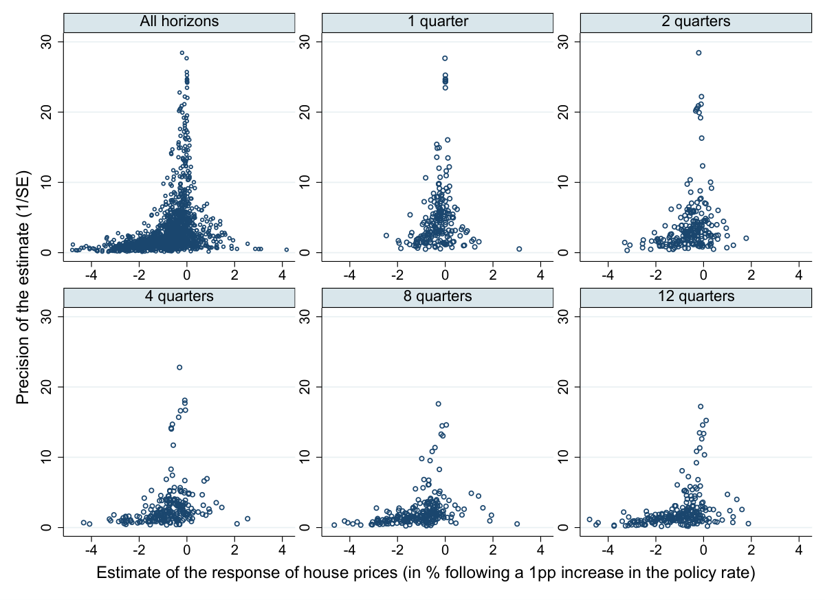
Corroborated by funnel asymmetry tests

Note that the slope is negative, the intercept is smaller than the reported mean effect:

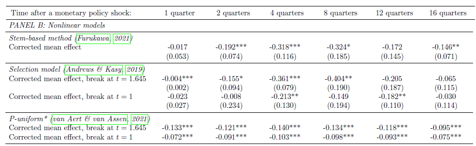
Nonliner tests also imply bias

Note that the corrected effect is smaller than the reported mean effect:

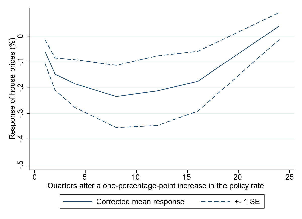
Mean impulse response beyond publication bias

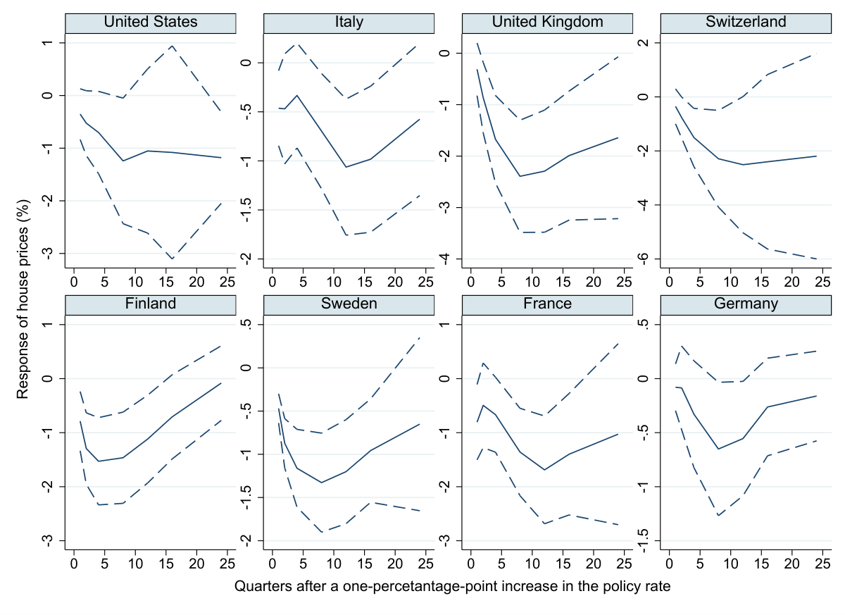
Cross-country heterogeneity

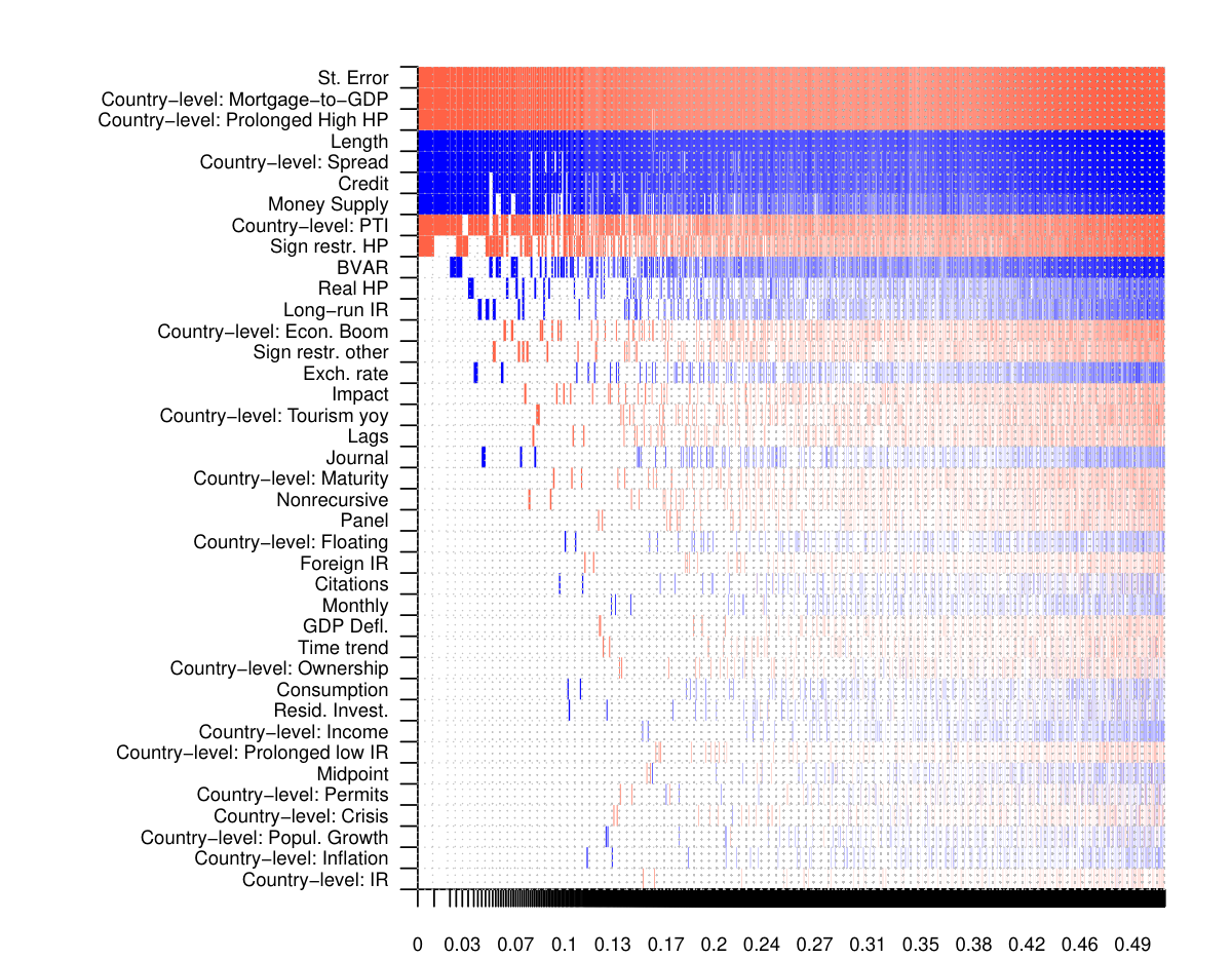
Estimation context

• Data characteristics: monthly, panel, length, age
• Specification characteristics: foreign IR, credit, consumption, res. invest., money supply, exch. rate, long-run IR, lags
• Estimation characteristics: BVAR, sign restr. HP, sign restr. other, nonrecursive
• Publication characteristics: citations, impact, published
• Country characteristics: mortgage-to-GDP, floating, maturity, IR, spread, prolonged high HP, PTI, crisis, prolonged low IR, tourism, income, inflation, popul. growth, permits, ownership

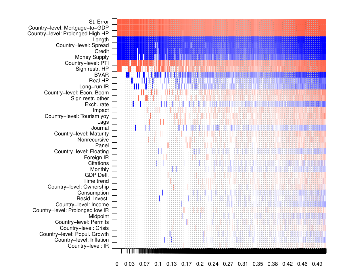
Bayesian model averaging

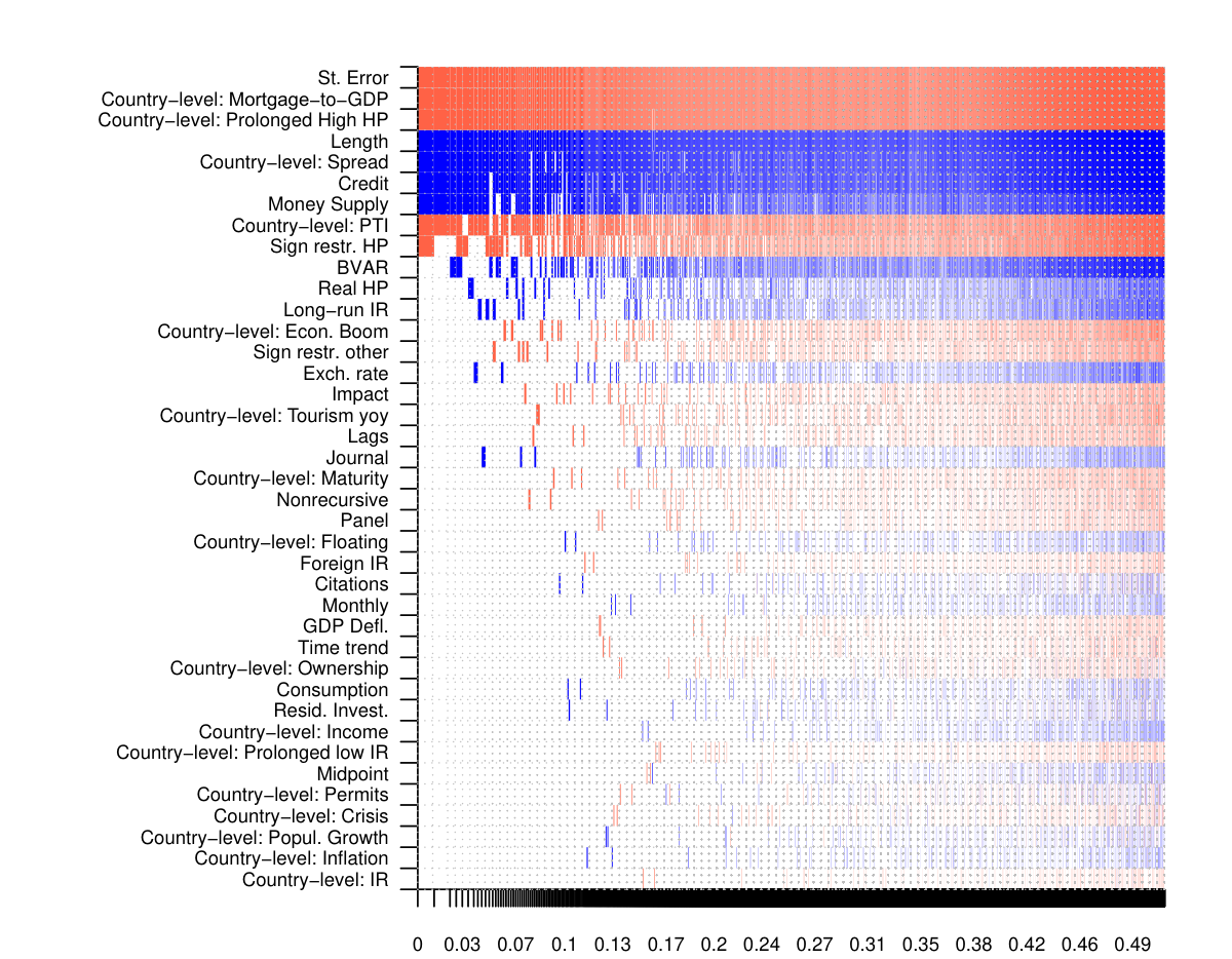
Best practice

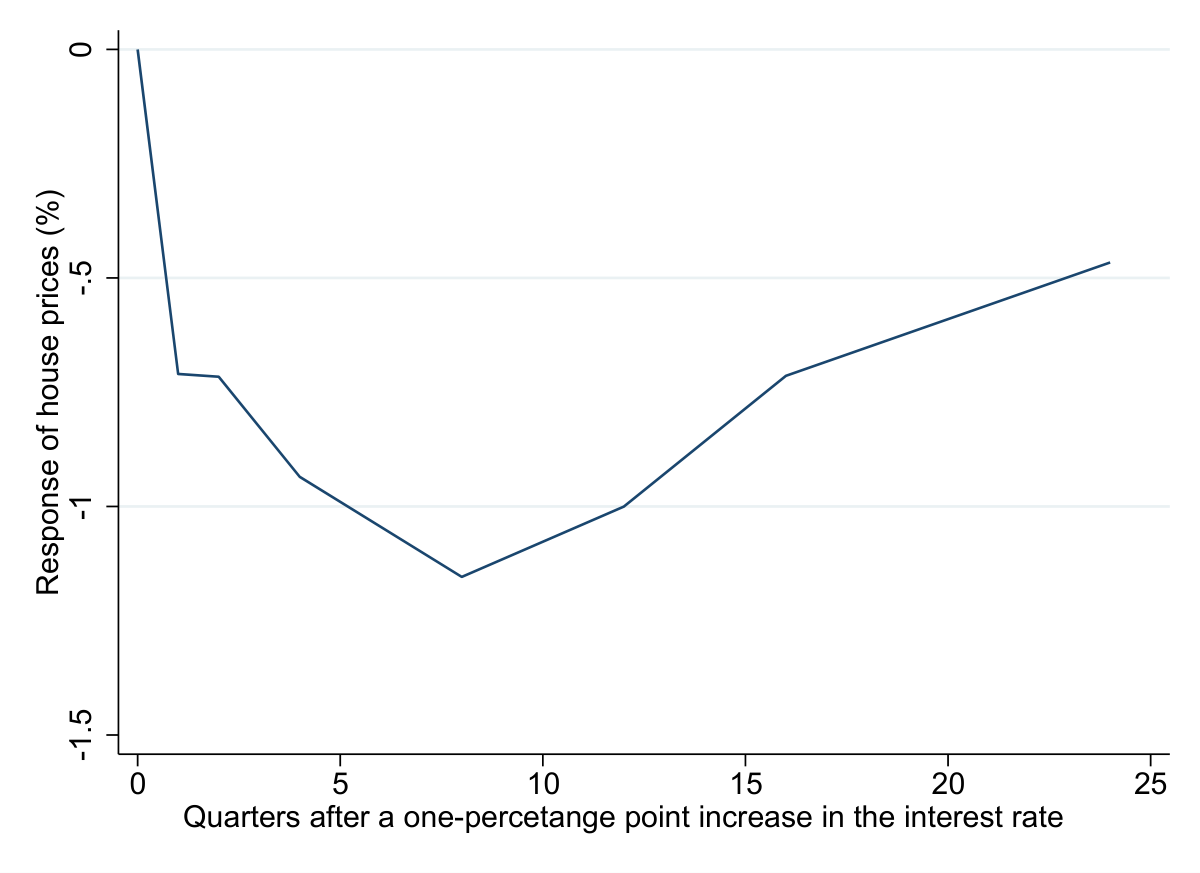
We construct a hypothetical ideal study: no publication bias (SE = 0), recent data, long series, nonrecursive identification, published, good journal, highly cited.

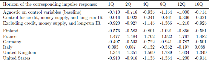
Impulse response implied by best practice

Results

1. Among 237 impulse responses from 37 studies, the mean decrease in house prices is 1.2% two years after a 1 pp. increase in the policy rate.
2. The mean is exaggerated because of publication bias.
3. Stronger transmission for i) more developed markets, ii) flatter yield curve, iii) house price boom.

www.meta-analysis.cz/house_prices

Example 3: Working while in school

• Hard to influence commonly cited determinants of educational outcomes: ability, ethnicity, gender, parental education and affluence
• But most students can decide whether or not to work
• How does that influence educational outcomes?
• Should you motivate your kids to work while in school?
• Mixed empirical results: from large negative to positive estimates
• 861 estimates from 69 studies

No consensus in the literature

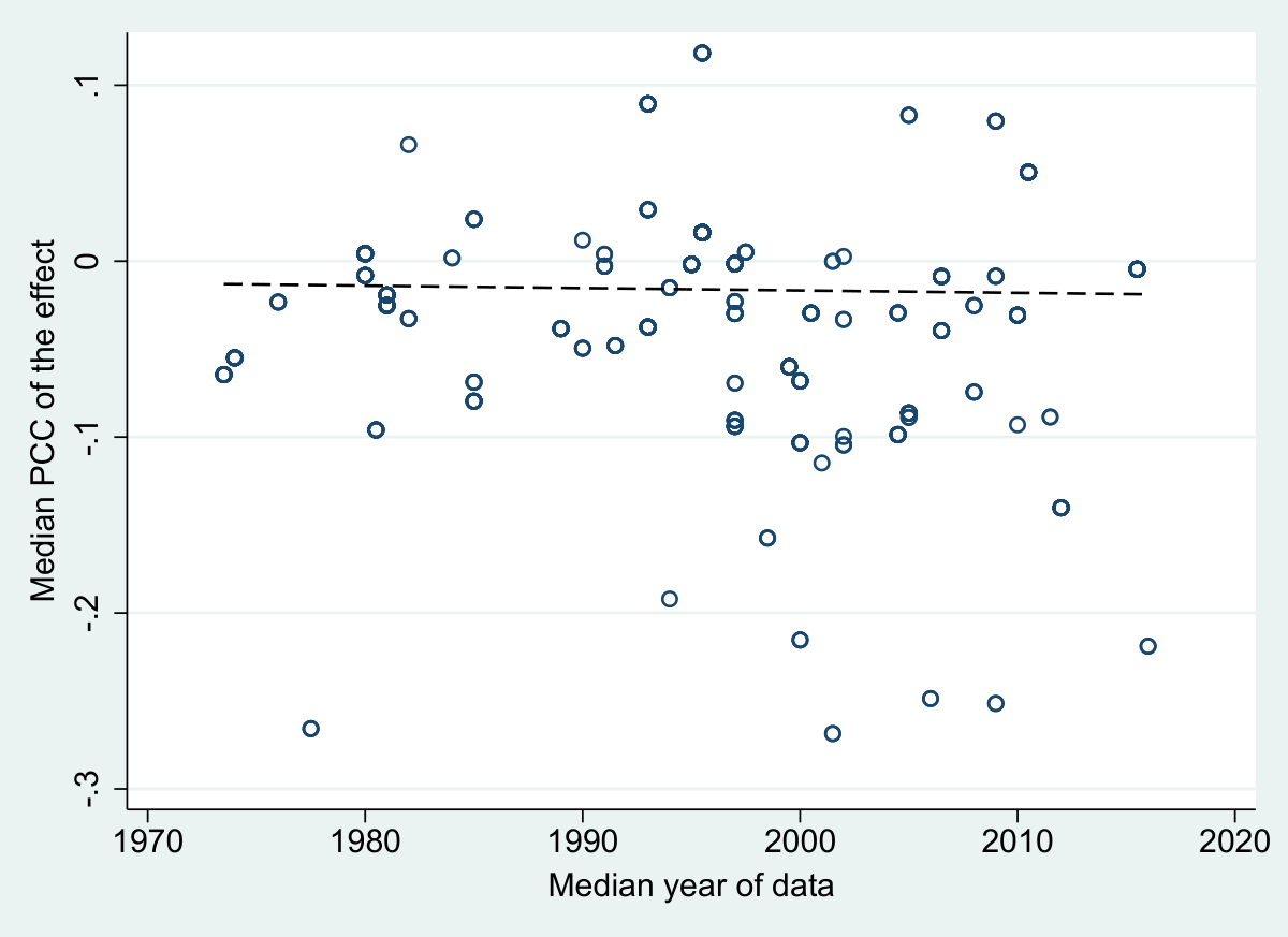
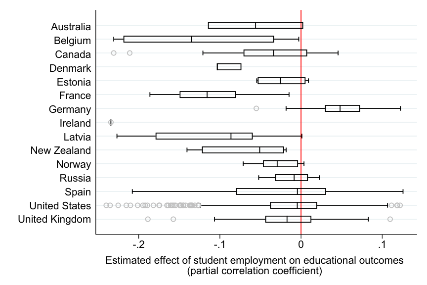
Negative for all countries except Germany

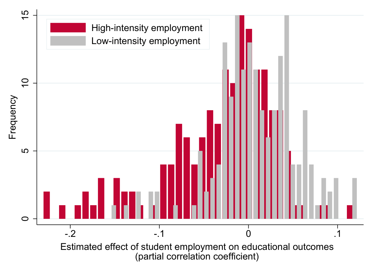
Work intensity clearly matters

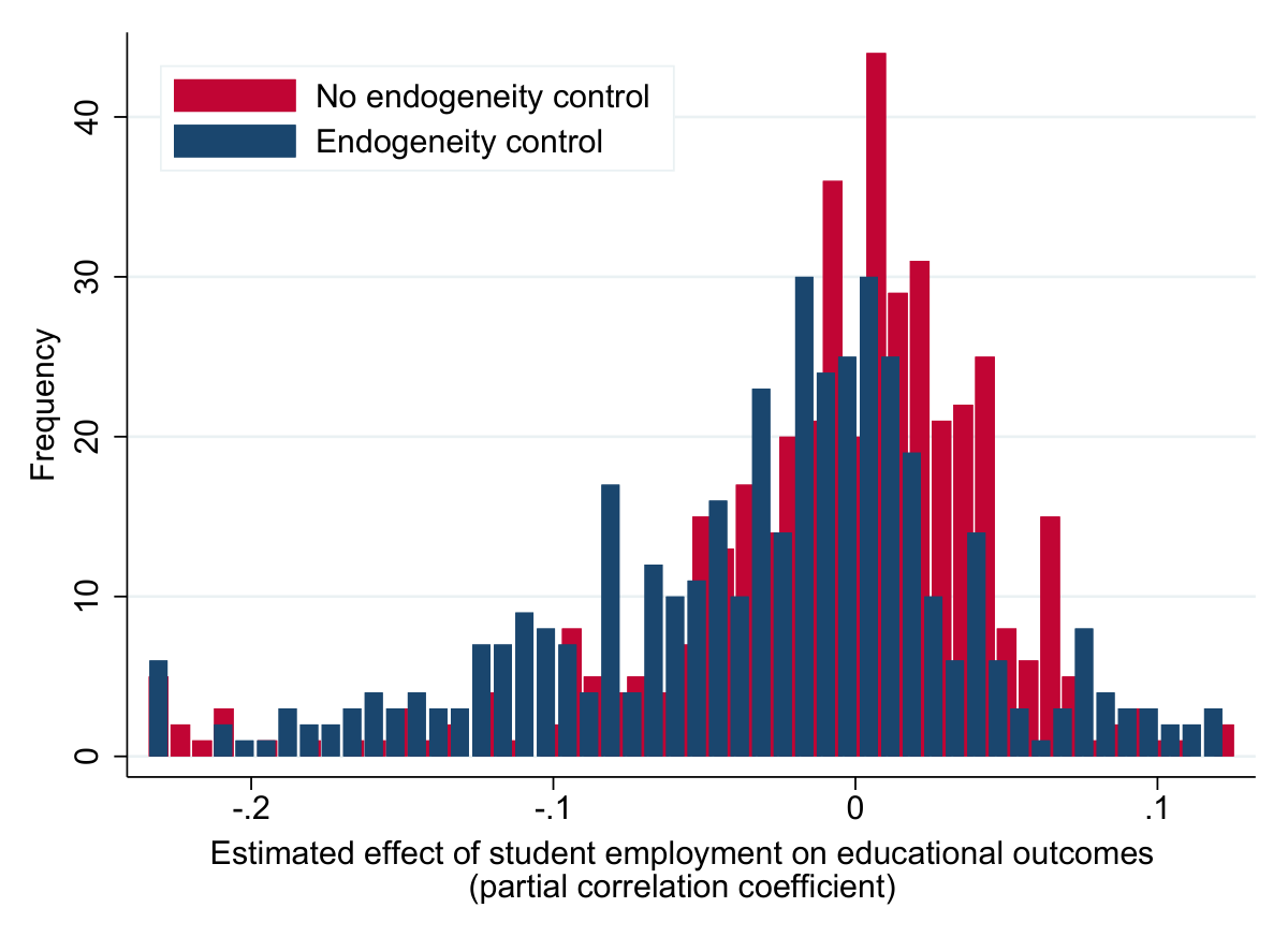
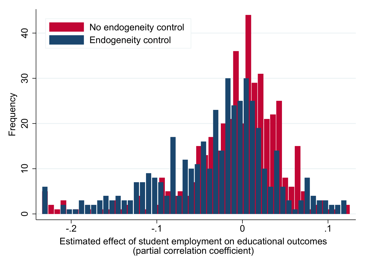
Endogeneity control is important

Little publication bias on average

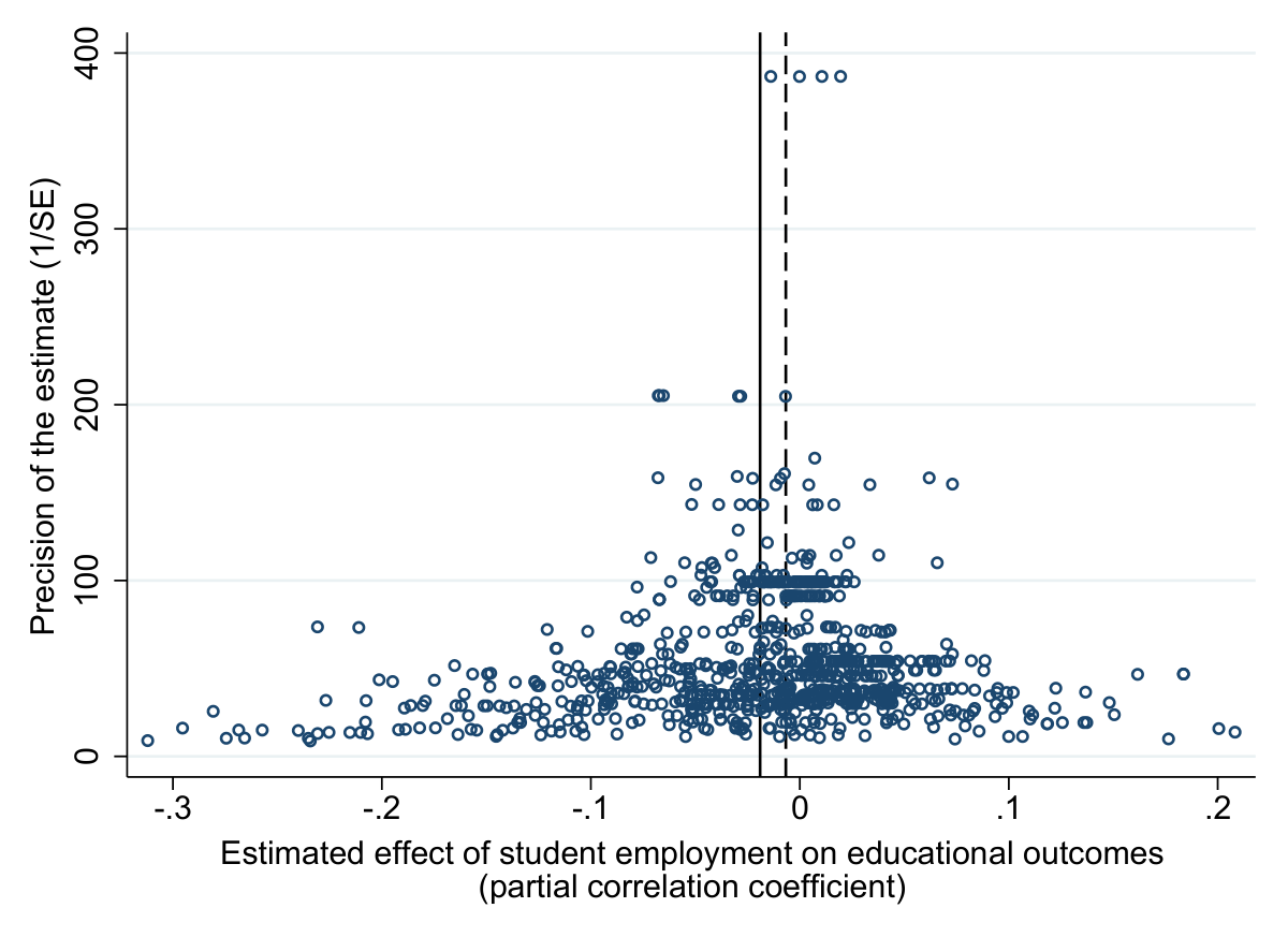
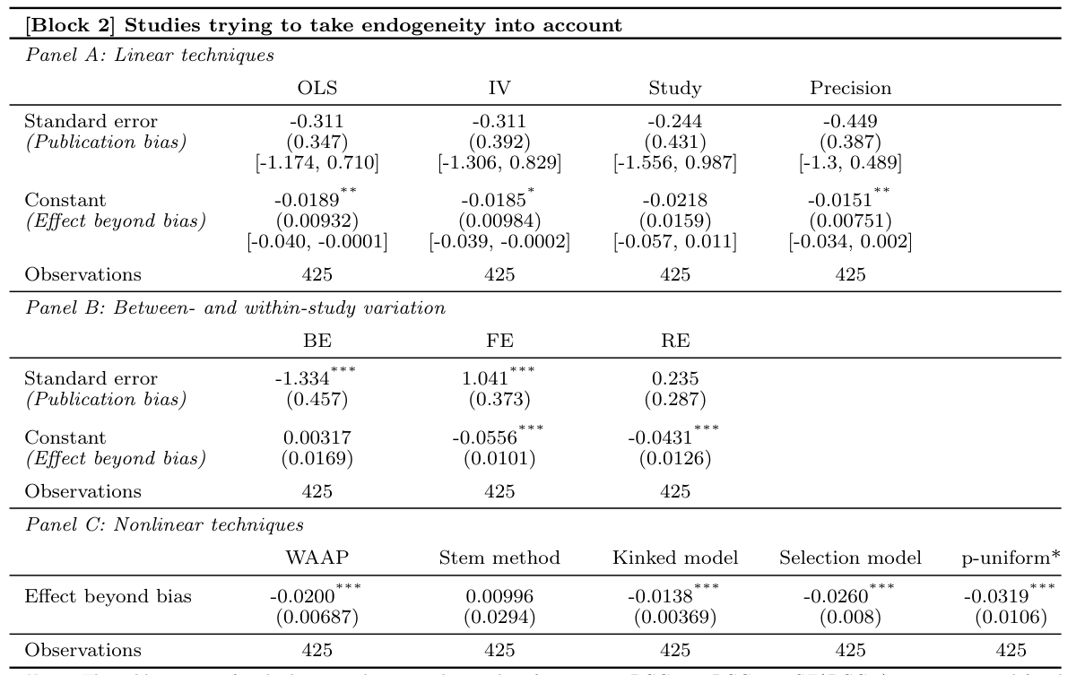
No bias in studies addressing endogeneity

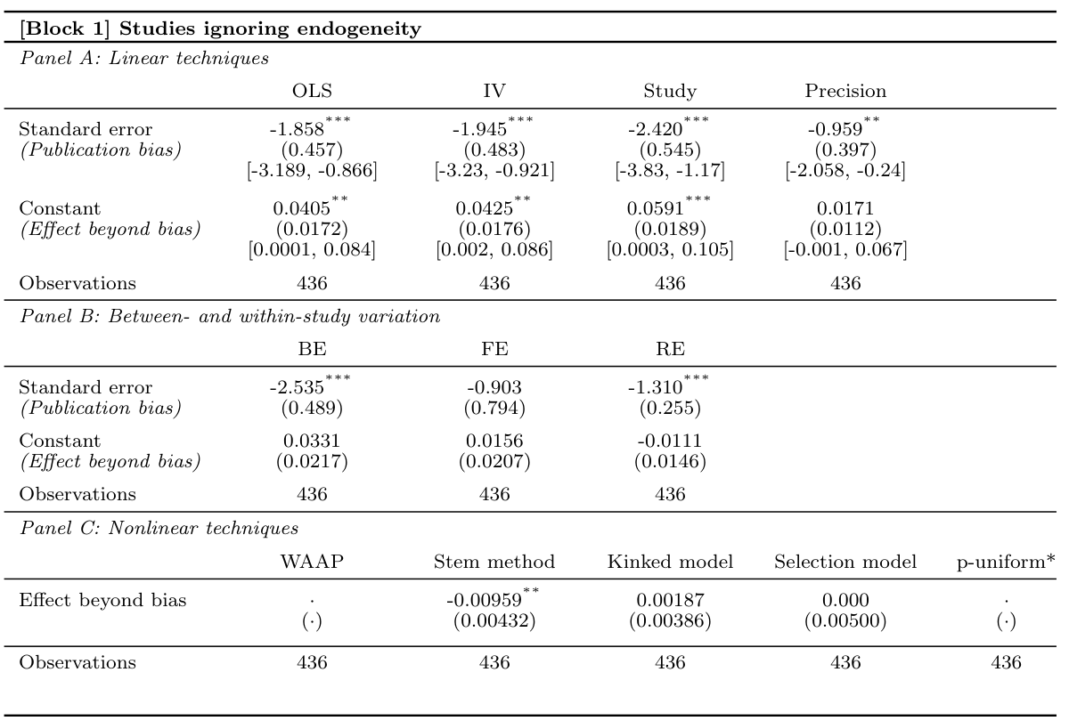
Strong bias in studies ignoring endogeneity

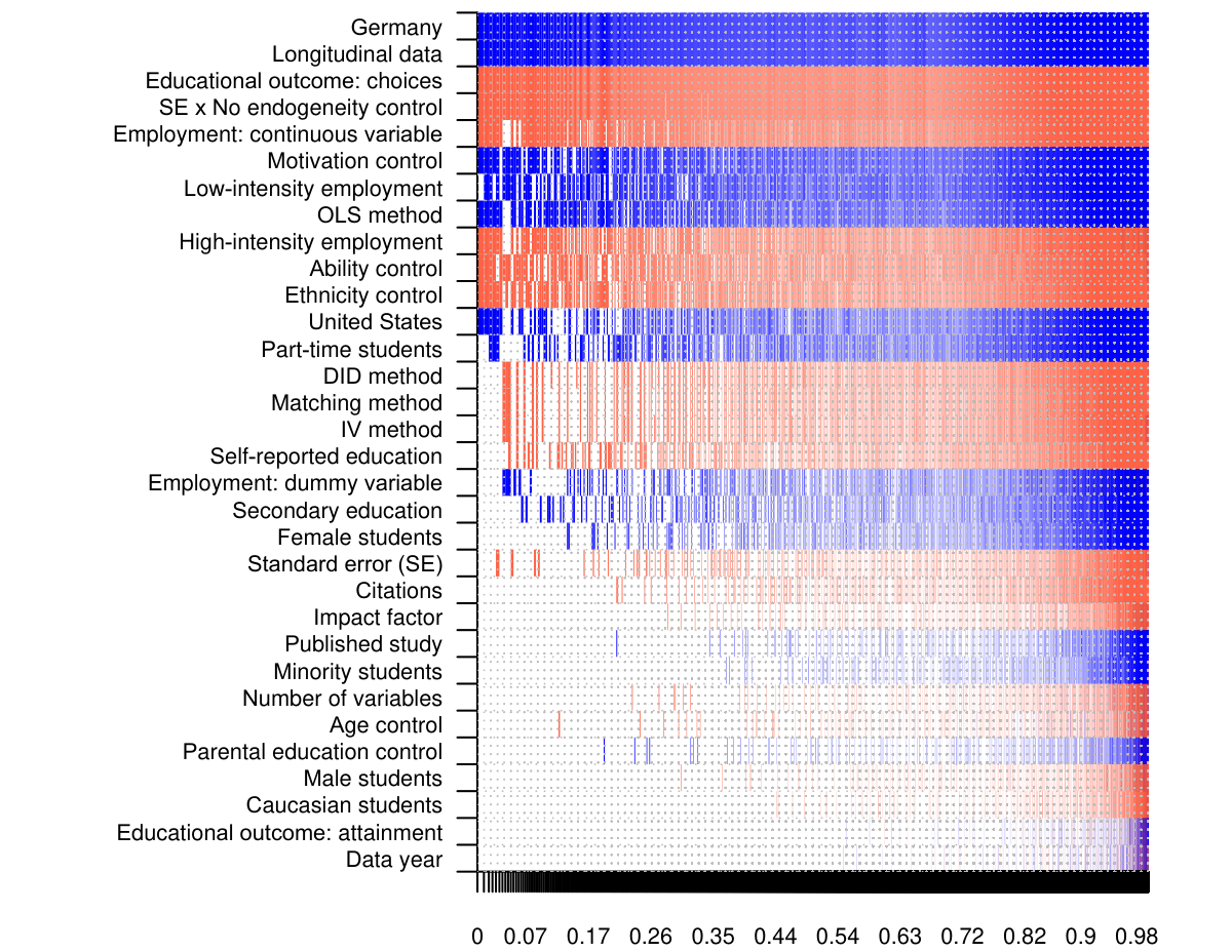
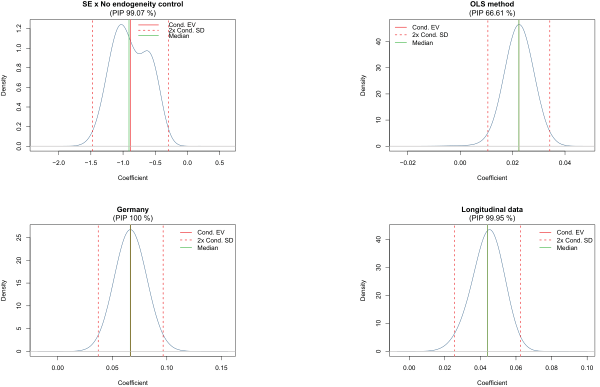
Model uncertainty; endogeneity control is key

Closer look: work intensity, measurement

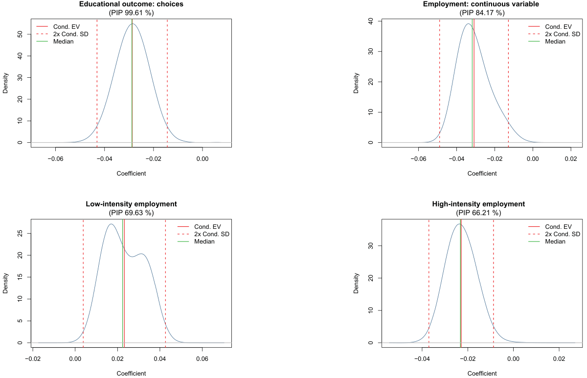
Closer look: endogeneity, panel data, Germany

Best practice estimates

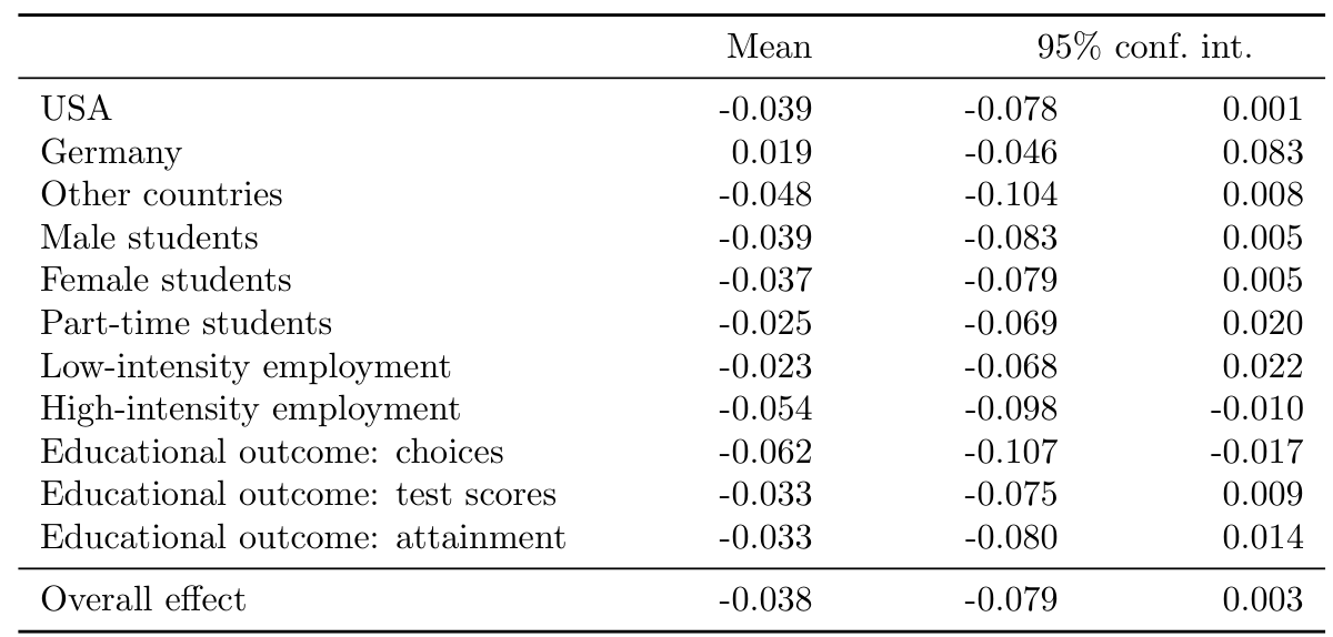
Results

1. Publication and endogeneity biases interact.
2. The corrected effect is negative but economically zero.
3. Effects negative for high-intensity work, positive for Germany.

www.meta-analysis.cz/students

Lecture 3: Literature Search

Choosing your topic

Prior to starting a meta-analysis, you should have at least a basic understanding of the field. Plus:

1. Policy interest
2. Missing publication bias analysis (in previous meta-analyses)
3. Missing heterogeneity analysis
4. Missing focus on economics
5. New methods

Inspiration

Motivation example 1

Motivation example 2

Motivation example 3

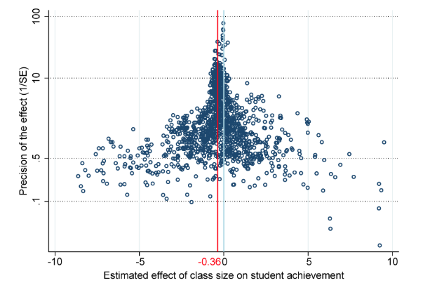
Motivation example 4

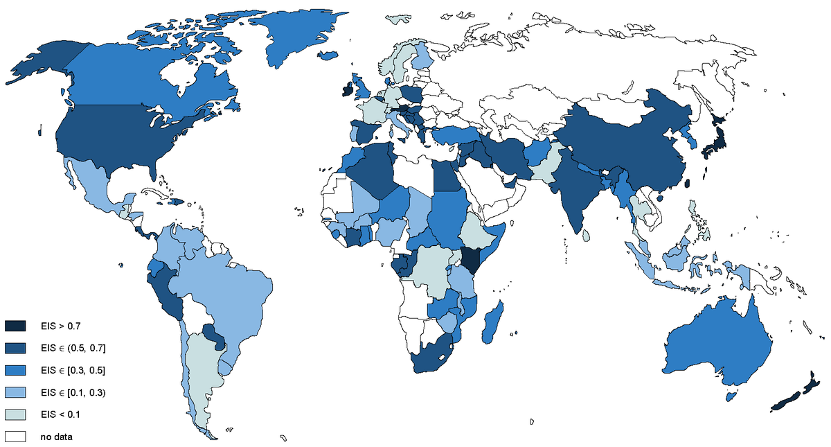
Motivation example 5

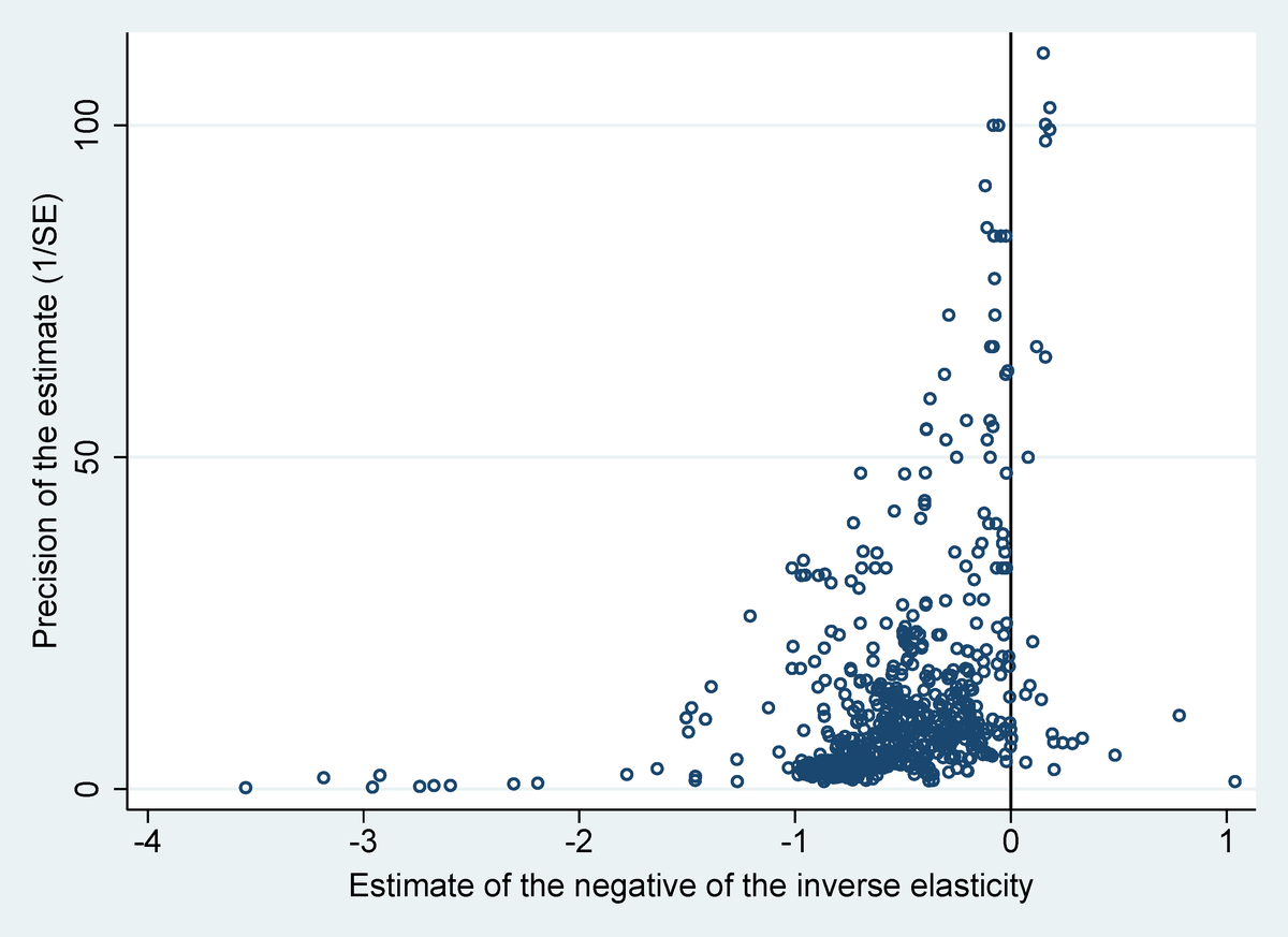
Motivation example 6

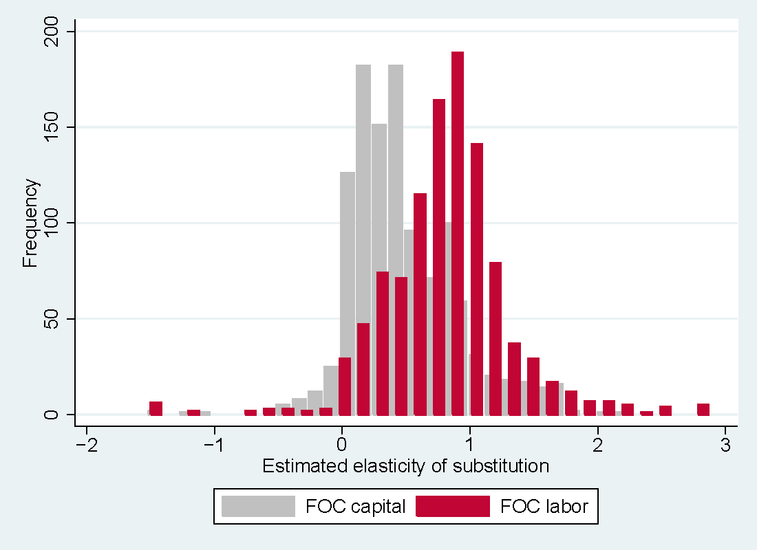
Google Scholar

Advantages:

• Full text, not just the abstract, title, keywords
• Inclusive
• Up-to-date

Disadvantages:

• Algorithm changes in time (replicability issues)
• Too many results
• Sometimes relevance unclear

Search steps

1. Find 5 most relevant studies (AI can help)
2. Design a Scholar query that shows the 5 studies near the top
3. Go through first 500 hits
4. Read abstracts
5. Download potentially useful studies
6. Skim them
7. Repeat the procedure for the most recent studies (last 3 years)

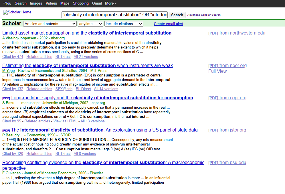
Search query 1

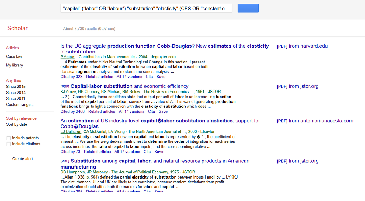
Search query 2

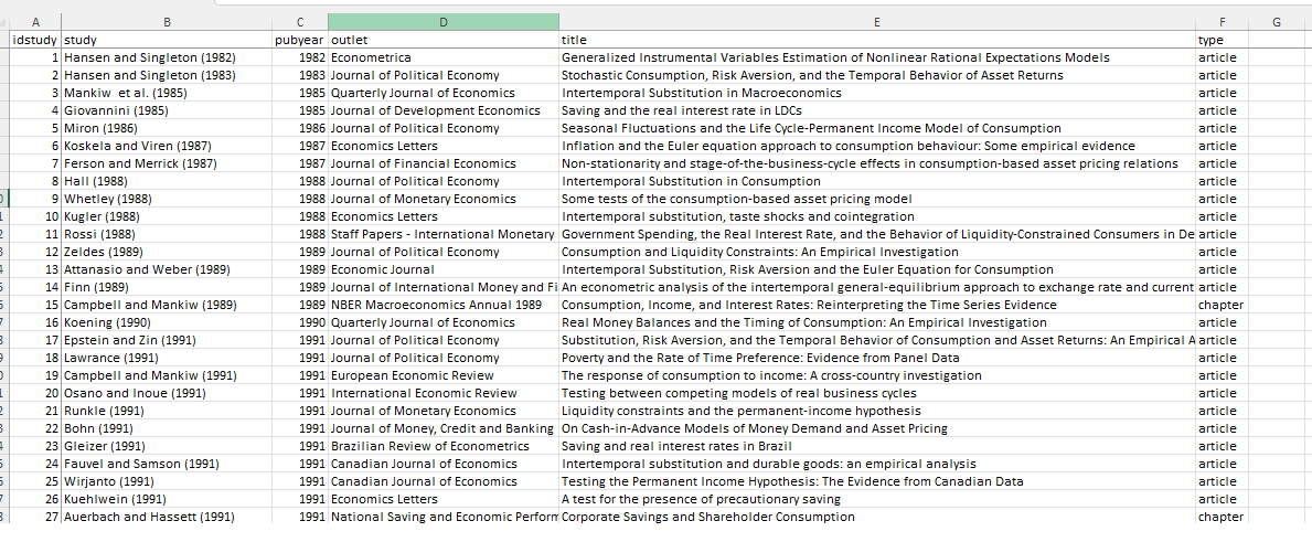
Primary studies

Snowballing

• No query is perfect
• Idea: cover studies not identified by the query but frequently mentioned in the literature
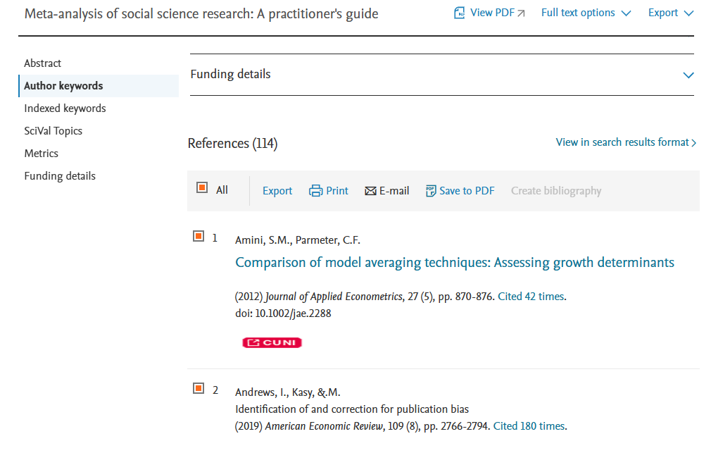
• For each primary study, download the list of references
• Inspect the 50 studies most frequently cited by the primary studies
• If you can use some of them, add them to your list

Snowballing example

Minimum requirements for meta-analysis

For modern meta-analysis techniques to work, you need at least:

1. 30 estimates
2. 10 studies
3. effect sizes
4. standard errors
5. sample sizes

Quality

• Some studies are published in poor journals or use weak identification. What to do?
• Option 1: exclude these studies ex ante. Not recommended.
• Option 2: include these studies with controls for journal quality and methodology. You can always exclude them as a robustness check.
• Note that some fields have standardized quality benchmarks (risk of bias)

Unpublished papers

• Try to collect all studies, published and unpublished
• If unfeasible, it is possible to focus just on published studies (fewer typos, peer-review)
• Including unpublished papers unlikely to alleviate publication bias
• Still too many papers? Recruit a co-author or use a random subset (last resort)

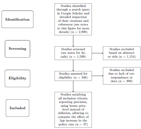
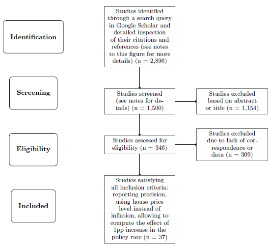
PRISMA: document your literature search

Lecture 4: Data Collection

Effects must be quantitatively comparable

What does it mean?

• When we compare estimates reported in Study 1 and Study 2, it must be clear which one is larger
• It must be clear how much larger it is
• t-statistics are not useful measures of effect size
• Regression coefficients are not comparable in general if studies use different units

Elasticities

x-elasticity of y: ε = ((∂ y)/y)/((∂ x)/x)

P-elasticity of Q: ε = ((∂ Q)/Q)/((∂ P)/P) if continuous

ε = ((Q_2 - Q_1)/Q_1)/((P_2 - P_1)/P_1) = (% change in quantity Q)/(% change in price P) if discrete

Elasticities can be recovered from regressing log(Y) on log(X).

Semi-elasticities, dollar values, std.dev. changes

• Semi-elasticity: effect of euro adoption on trade, effects of foreign investment on domestic productivity, effects of borders on trade
• Dollar values: statistical value of life, social cost of carbon
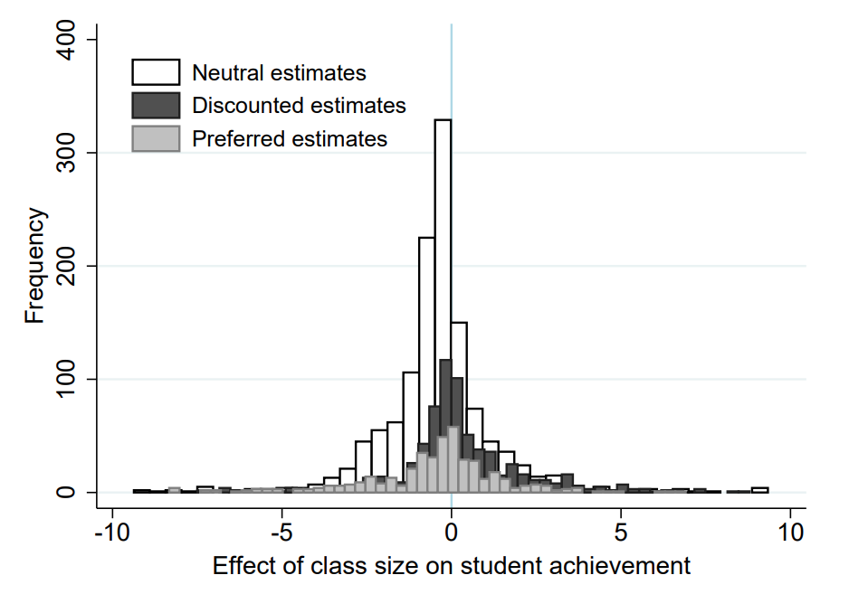
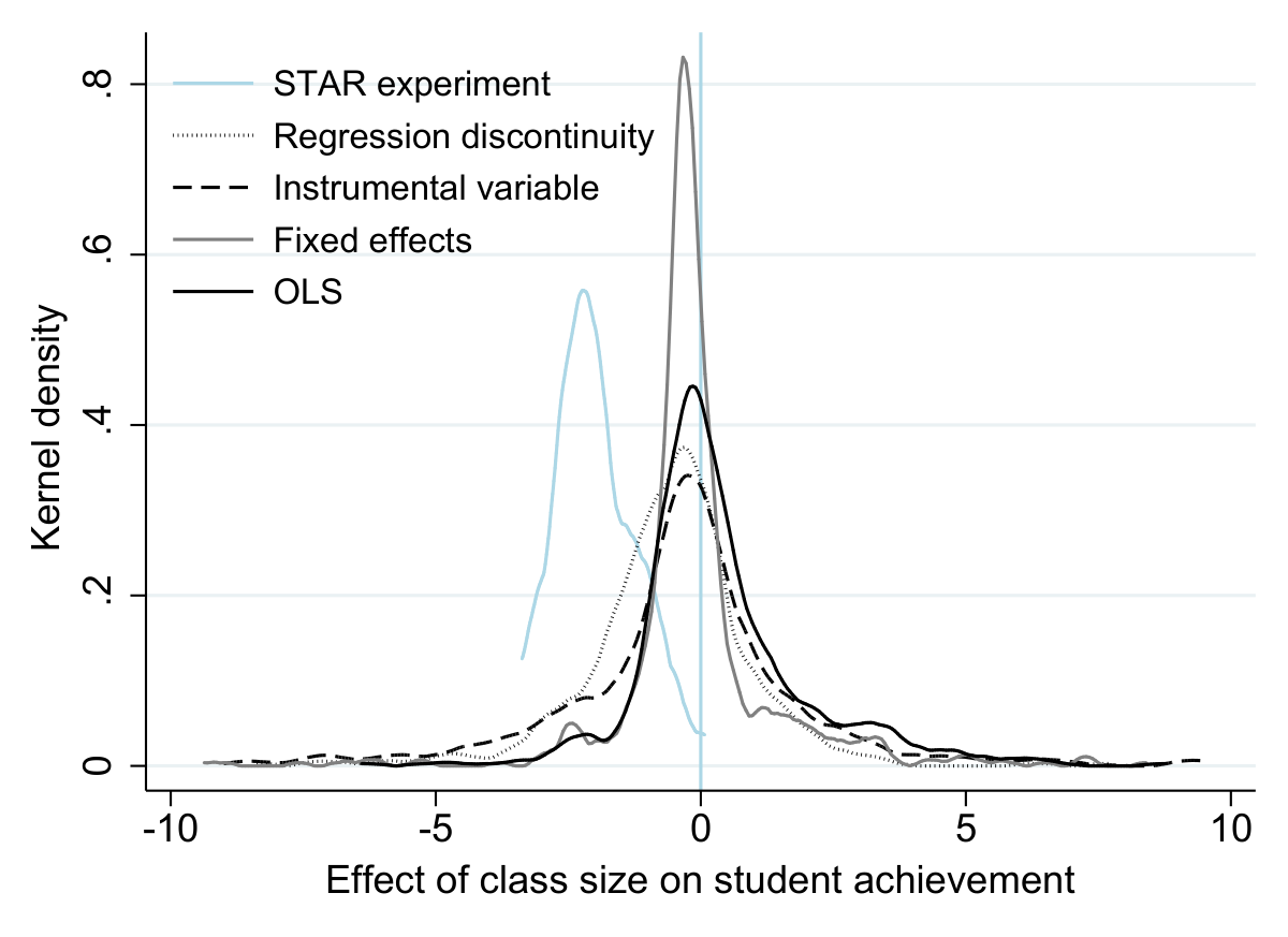
• Std.dev. changes: effect of class size on student test scores. What to do here?
• Class size is measured the same way in all studies (number of kids).
• Test scores are measured differently.
• Solution: By how many standard deviations do test scores improve if we decrease class size by 10 students?

Standardized mean differences

θ = (μ_1 - μ_2)/σ, where μ_1 is the mean for one population, μ_2 is the mean for the other population, and σ is a standard deviation based on either or both populations.

• Very popular in psychology, not much used in economics. Why?
• Generally we need an experiment: treatment group, control group.
• In economics we often focus on observational research.
• For many questions the treatment and control are not binary classifications (we look at the intensity of treatment)

Partial correlation coefficients

Example: tuition fees and university enrollment. Ideally, we would need price elasticities of demand (PED), but many studies are not log on log.

So we transform the estimates to partial correlations using t-statistics and degrees of freedom:

PCC(PED)_ij = (T(PED)_ij)/(√(T(PED)_ij^2 + DF(PED)_ij)).

PCC caveats

• Last resort: can be used almost always, but we lose a lot of information
• Difficult to interpret (some guidelines provided by Doucouliagos, 2011)
• Statistical problems for meta-analysis methods (but this is the case also for SMD)
• Include robustness checks: e.g. a subsample of elasticities in the case of tuition fees and university enrollment

Collect all estimates

Standard errors

• Absolutely crucial for meta-analysis
• If not reported directly, can be computed from t-statistics or p-values
• Last resort: approximation based on within-study variation (Matousek et al. 2022)
• Interactions, transformations: delta method

Delta method

Based on Taylor series expansion. Basic formula:

Var(Y) = Var(f(X)) ≈ [f'(μ_X)]^2 Var(X).

Example: Suppose Y = X^2. Then f(x) = x^2 and f'(x) = 2x, so that: Var(Y) ≈ [2μ_X]^2 Var(X) = 4μ_X^2σ_X^2.

Example: Suppose Y = 1/X. Then f(x) = 1/x and f'(x) = -1/x^2, so that: Var(Y) ≈ [(-1)/μ_X^2]^2 Var(X) = σ_X^2/μ_X^4.

Graphical estimates, measurement error

Outliers

What to do with outliers?

• No consensus
• Approach 1: omit very large effects (and standard errors), e.g. more than 3 standard deviations away from the mean
• Approach 2: run robust meta-regression or use tools for outlier detection in regression
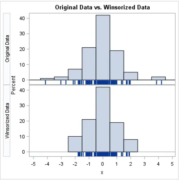
• Approach 3: use winsorizing (my personal preference)
• Always report robustness checks

Winsorization

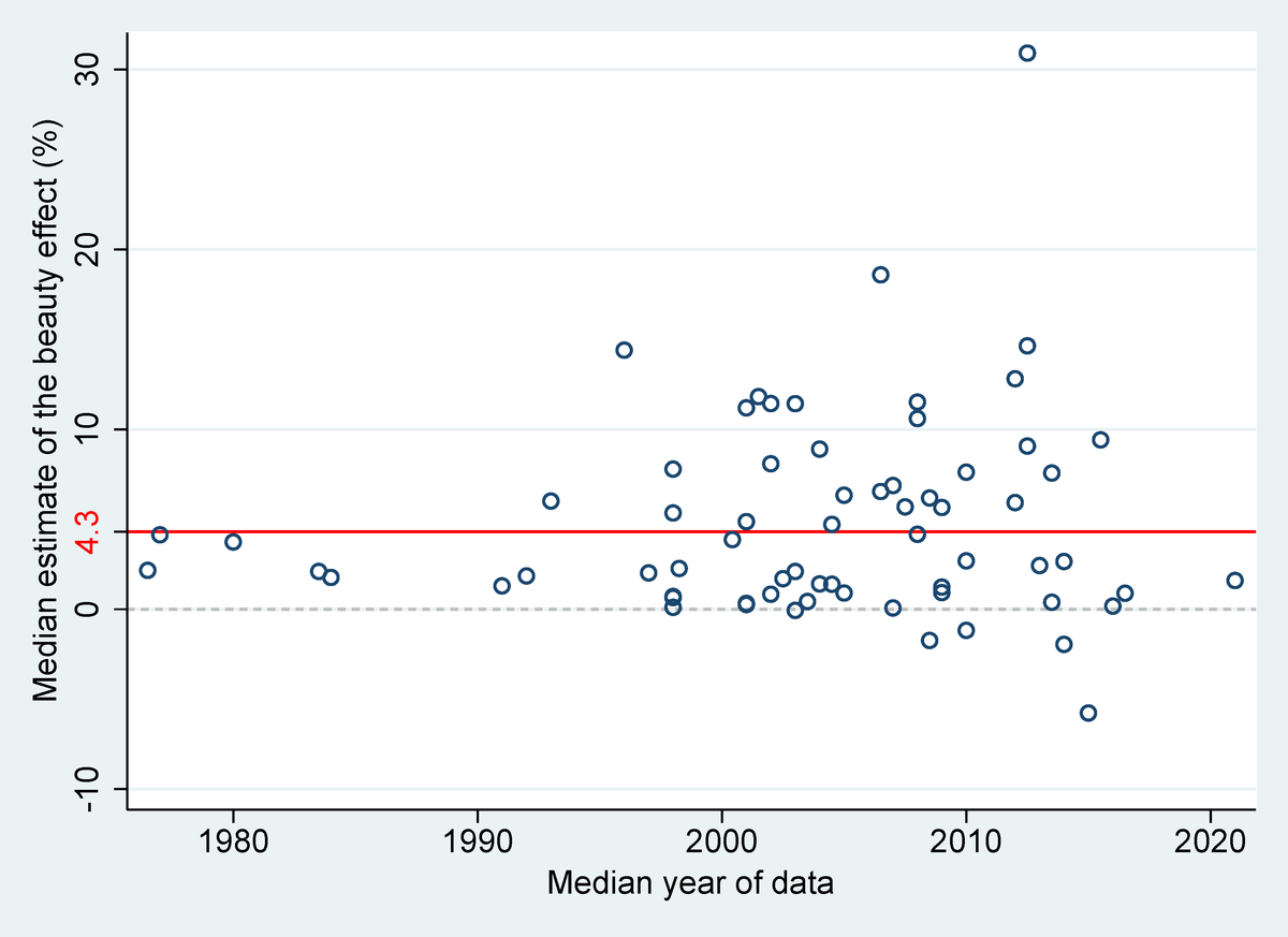
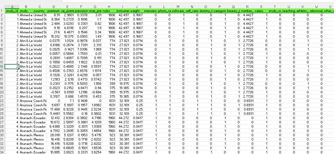
Reflecting context: the effect of beauty on success

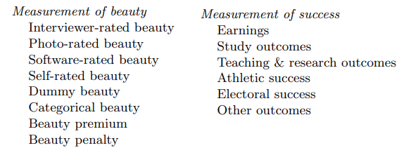
Measurement

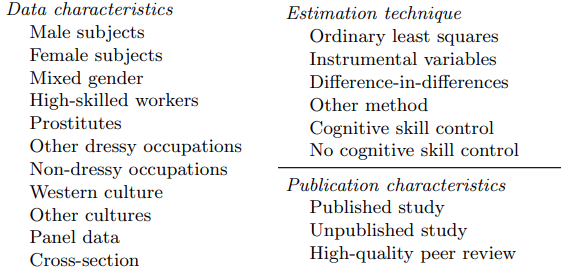
Data, estimation, publication

Artificial intelligence and context

• Can be useful for identifying key aspects in which studies vary
• Do not trust AI replies too much, but you can use it at various stages to generate ideas about potential explanatory variables
• You can use it to check whether you missed an important variable

Value added

• Meta-analysis can be used to test hypotheses that primary studies cannot investigate
• Example: the effect of daylight saving time on energy consumption
• Individual studies have data for individual countries (or provinces)
• In meta-analysis, we have data for dozens of countries
• We can investigate the sources of cross-country differences

DST savings and latitude

House prices and monetary policy

Lecture 5: Basic Meta-Analysis Tools

Mean, median, something else?

• Simple mean of reported estimates: often good starting point
• But inefficient, affected by outliers, publication bias
• Median: surprisingly robust to most problems in meta-analysis
• Classical meta-analysis approach: use inverse variance as the weight

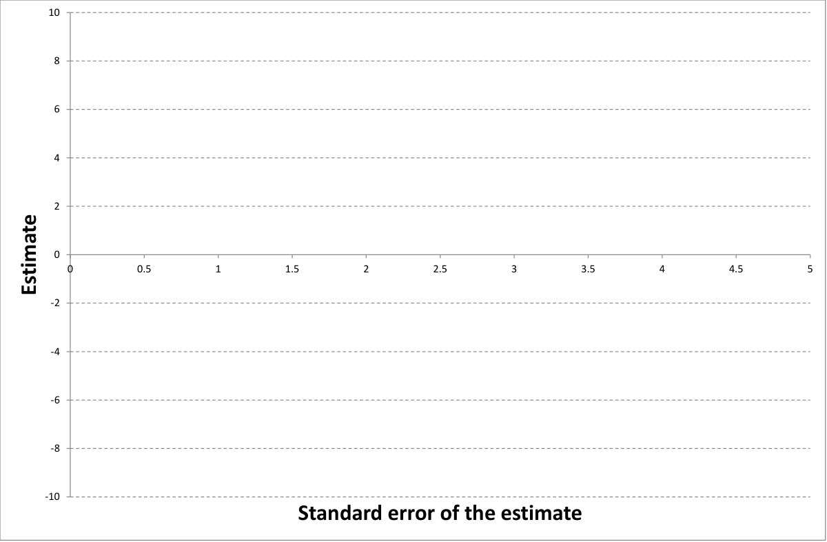
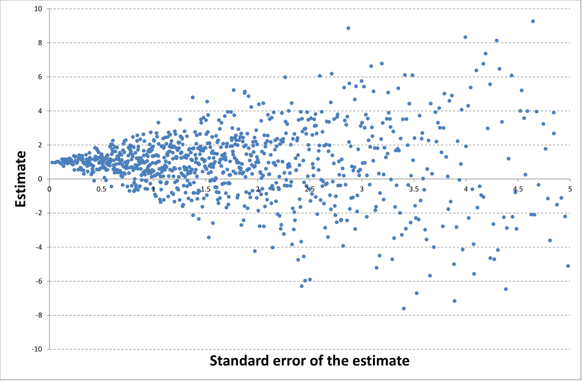
More precision -> more weight

More precision -> more weight

More precision -> more weight

Fixed effect

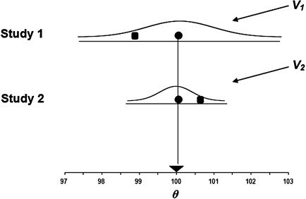
Fixed effect

Y_i = θ + ε_i, (1); V_i = σ^2/n, (2); W_i = 1/V_i, (3); M = (Σ_(i=1)^k W_i Y_i)/(Σ_(i=1)^k W_i), (4); V_M = 1/(Σ_(i=1)^k W_i). (5)

FE vs. UWLS: point estimate

• Both methods yield the same point estimate: θ̂ = (Σ w_i θ_i)/(Σ w_i), w_i = 1/σ_i^2
• Key difference: Variance estimation.

Method | Point Estimate
Fixed-Effect (FE) | θ̂ = (Σ w_i θ_i)/(Σ w_i)
UWLS | θ̂ = (Σ w_i θ_i)/(Σ w_i)

Same estimate, different variance!

FE vs. UWLS: variance

Feature | Fixed-Effect (FE) | UWLS
Assumption | Identical θ | Allows heterogeneity
Variance formula | 1/(Σ w_i) | (Σ w_i (θ_i - θ̂)^2)/(Σ w_i)
Variance components | Within-study only | Within + between-study
Robustness | Sensitive to misspecification | More robust

FE underestimates variance if heterogeneity exists!

Correction. The UWLS variance of the pooled estimate is Σ w_i (θ_i - θ̂)^2 / ((k - 1) Σ w_i); the table leaves out the factor k - 1. This is the formula for independent estimates: with several estimates per study, use standard errors clustered by study.

Fixed effect

Random effects

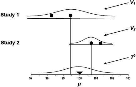
Random effects

Y_i = μ + ξ_i + ε_i, (1); V_i = σ^2/n, (2); W_i = 1/(V_i + T^2), (3); M = (Σ_(i=1)^k W_i Y_i)/(Σ_(i=1)^k W_i), (4); V_M = 1/(Σ_(i=1)^k W_i). (5)

Estimating τ^2 in random-effects model

Between-study variance τ^2 accounts for heterogeneity across studies. Common estimators:

• DerSimonian-Laird (DL): τ^2_DL = (Q - (k - 1))/C, C = Σ w_i - (Σ w_i^2)/(Σ w_i). Simple, but underestimates τ^2 when k is small.
• Restricted Maximum Likelihood (REML): max_τ^2 Σ log (w_i^* + τ^2) + Σ ((y_i - θ̂)^2)/(w_i^* + τ^2). More accurate, default in software.

Rule of thumb: Use REML unless simplicity is needed!

Correction. The REML line is not the restricted likelihood. REML chooses τ^2 ≥ 0 to minimise Σ log(v_i + τ^2) + log Σ W_i + Σ W_i (y_i - θ̂)^2, where v_i are the within-study variances, W_i = 1/(v_i + τ^2) and θ̂ is the weighted mean; software solves this numerically. A negative DL estimate is set to zero.

Random effects

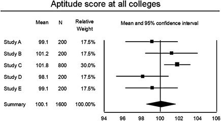
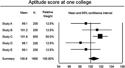
Forest plot

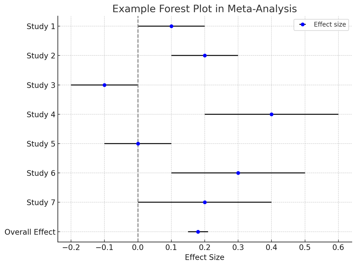
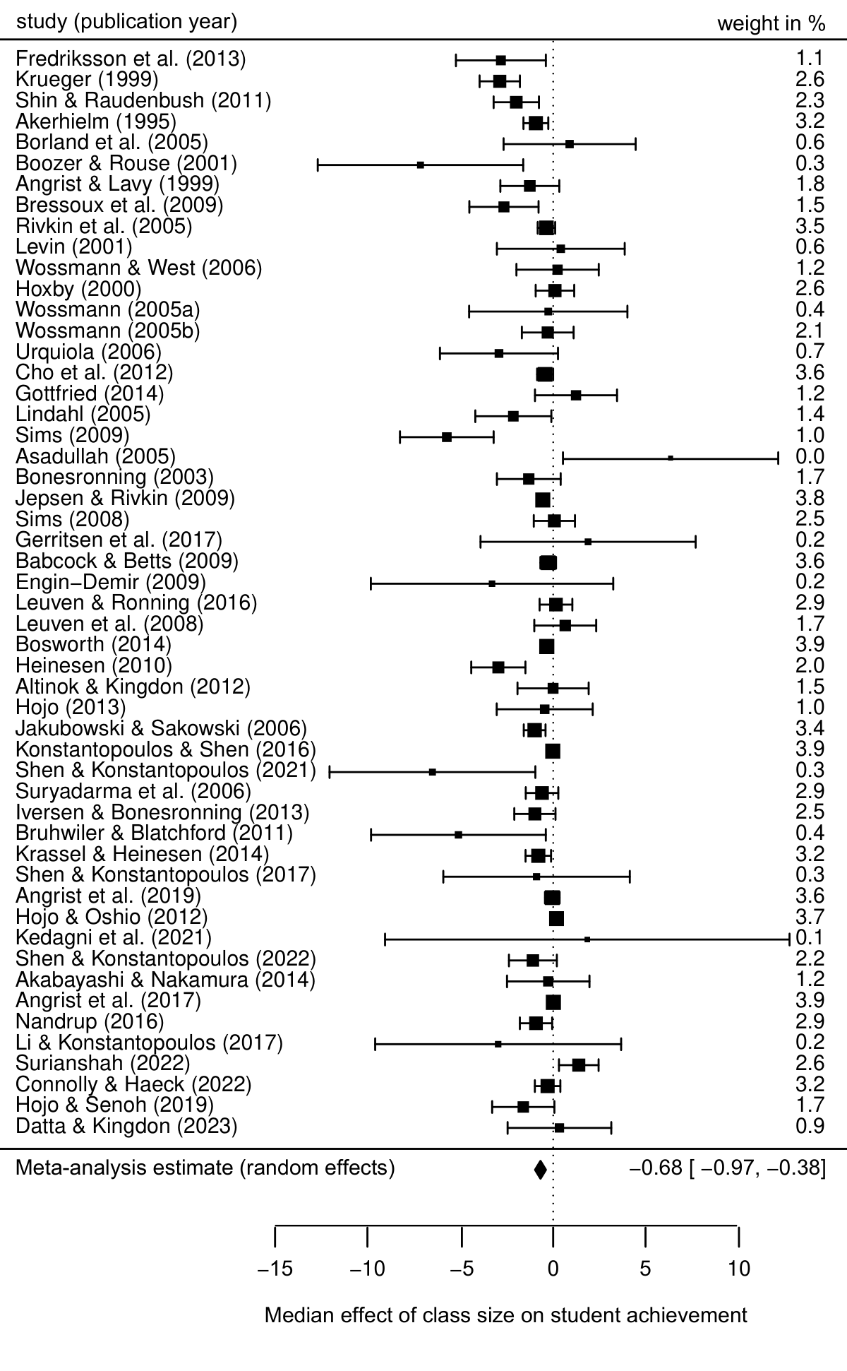
Forest plot

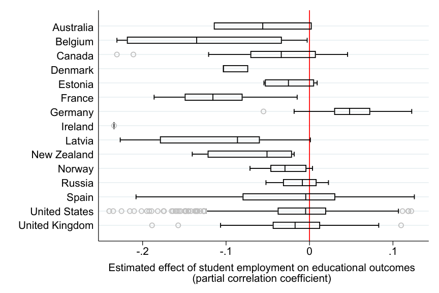
Box plot

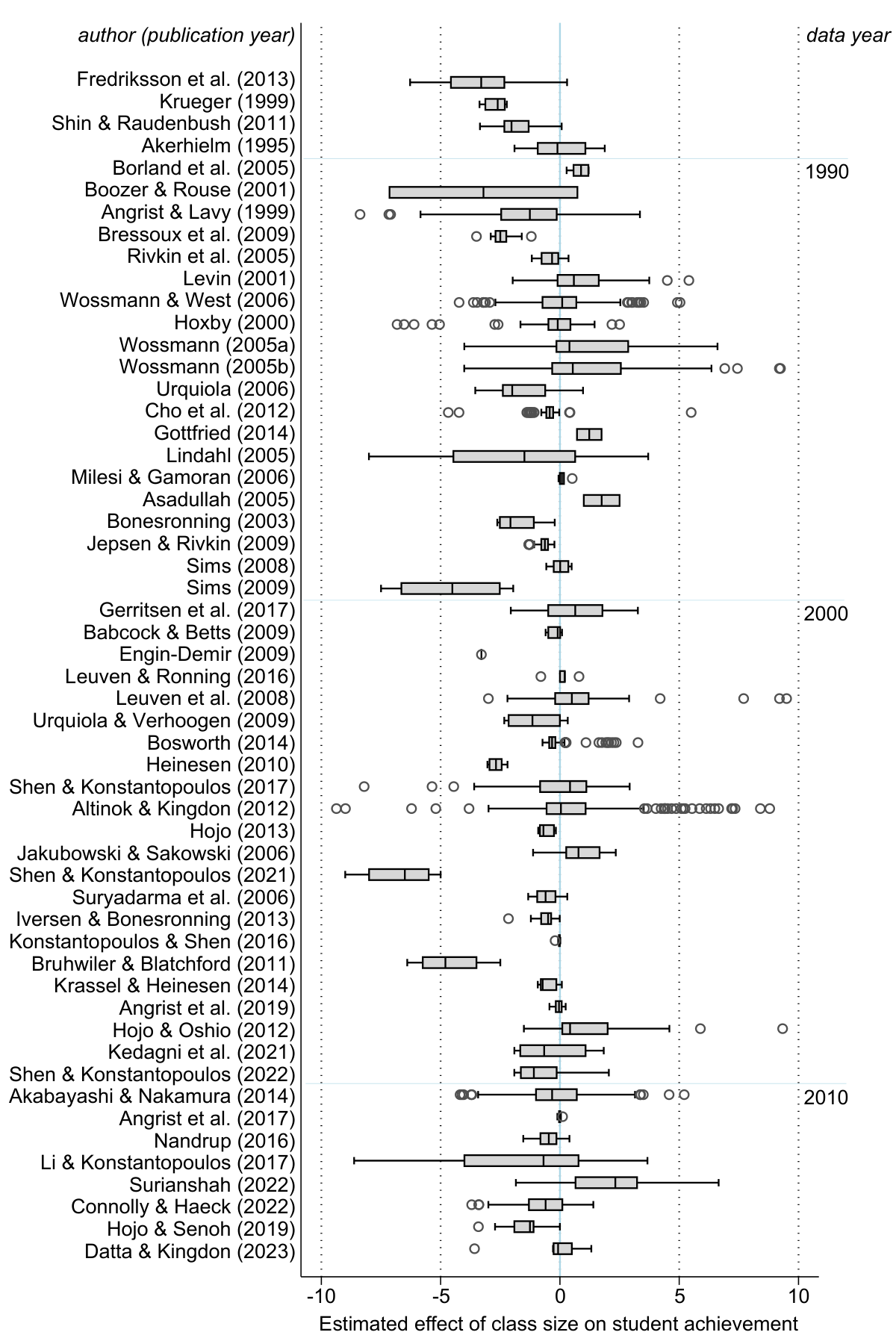
Box plot

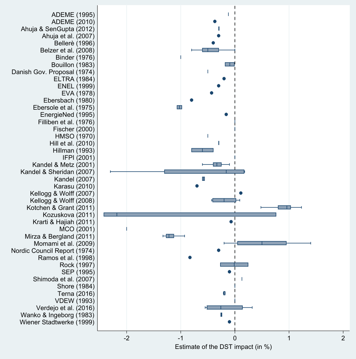
Box plot

Histogram

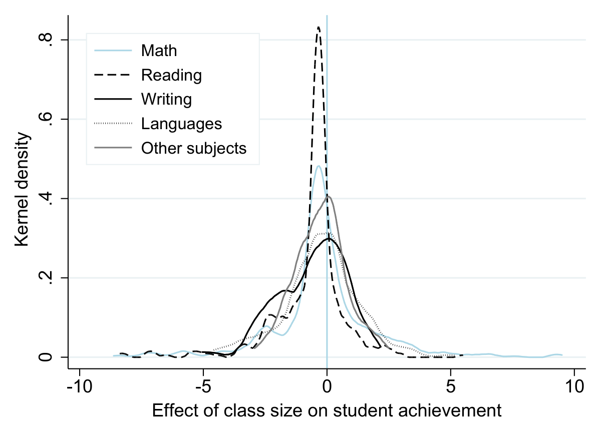
Histogram

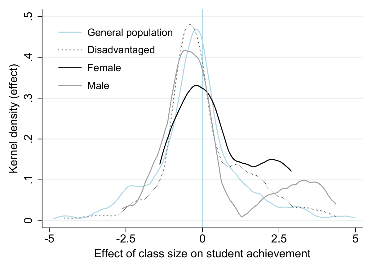
Histogram

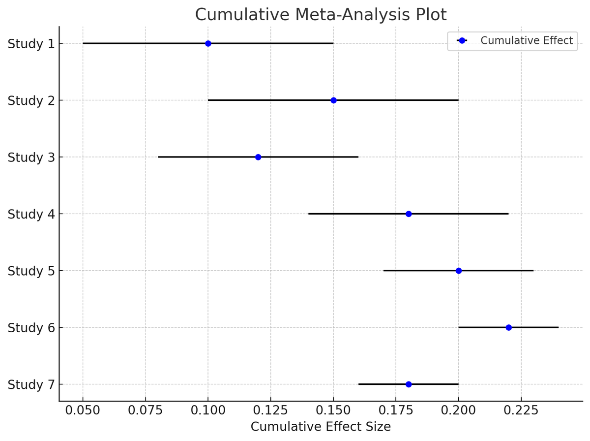
Cumulative meta-analysis plot

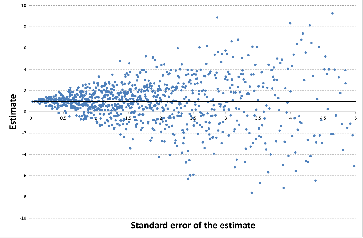
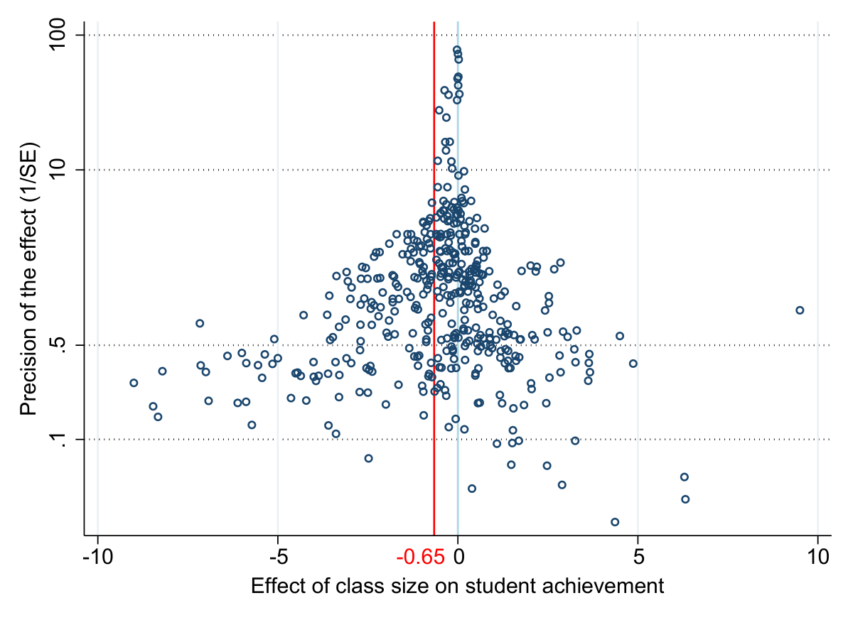
Funnel plot (topic of the next lecture)

Lecture 7: Publication Bias

Intuition

Intuition

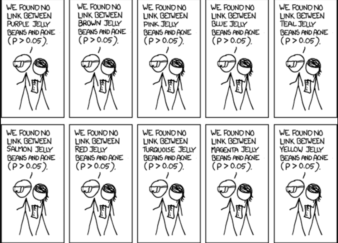
Intuition

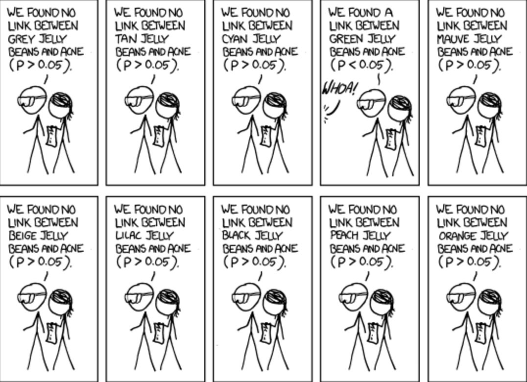
Intuition

Paxil scandal

• Background:
  • Paxil (paroxetine): Antidepressant approved for adolescents, developed by GlaxoSmithKline (GSK).
  • Study 329 (1998-2001): Clinical trial funded by GSK to test Paxil's safety and efficacy in adolescents.
• What Happened?
  • Published study claimed Paxil was "well-tolerated and effective."
  • Internal documents later revealed:
    • Negative results (e.g., increased suicidal ideation) were downplayed.
    • Positive outcomes were selectively reported.

Correction. The FDA never approved paroxetine for patients under 18: it was approved for adults and promoted for adolescent depression. Study 329 ran from 1994 to 1998 and was published in 2001; the independent reanalysis appeared in 2015.

Paxil scandal

• Discovery of Bias:
  • Legal proceedings in 2012 forced disclosure of internal data.
  • Independent reanalysis of Study 329 showed:
    • No significant benefit over placebo.
    • Serious safety concerns (e.g., suicidal ideation).
• Key Lessons:
  • Publication bias can harm patients and public trust.
  • Highlights the need for:
    • Transparency in research data.
    • Independent replication and reanalysis.

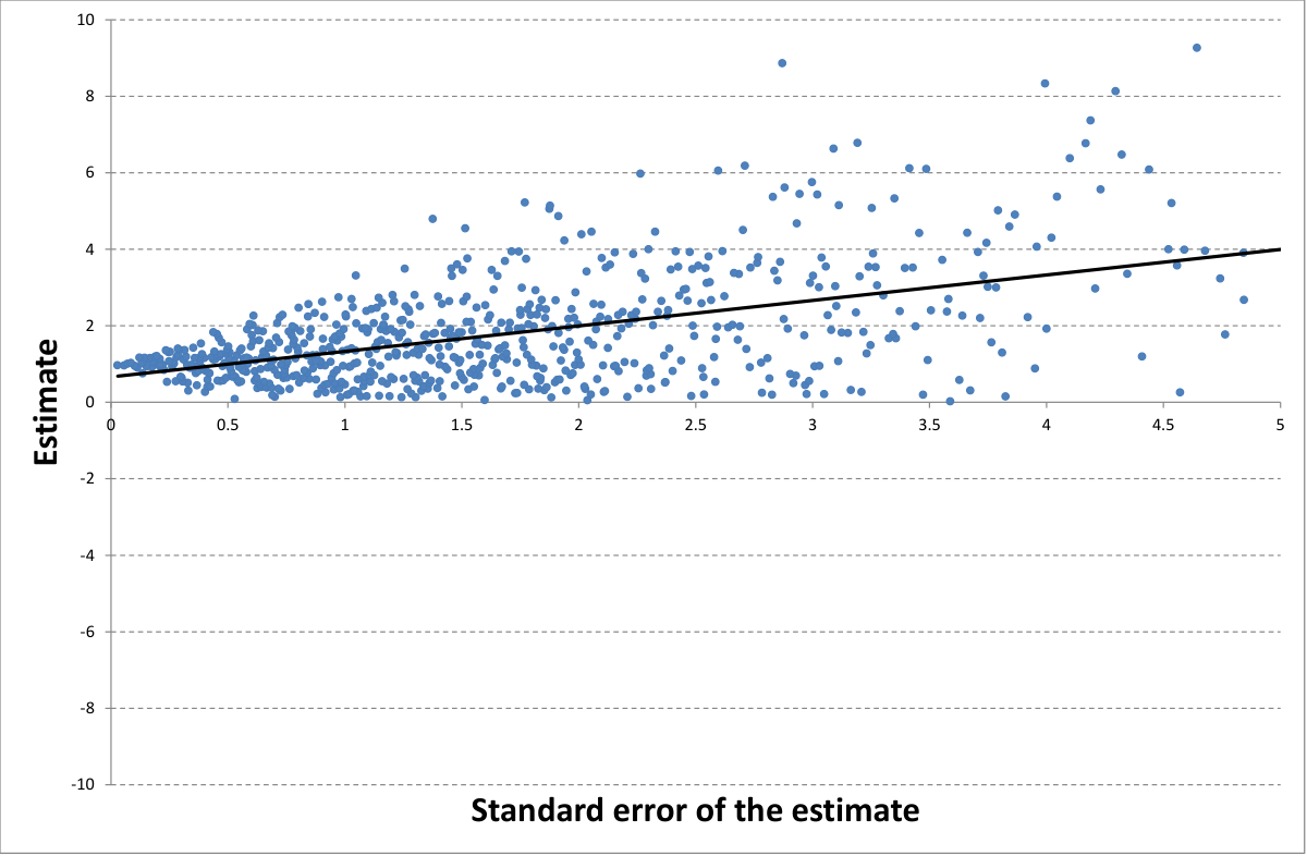
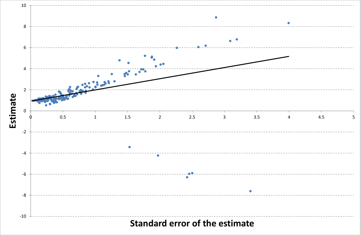
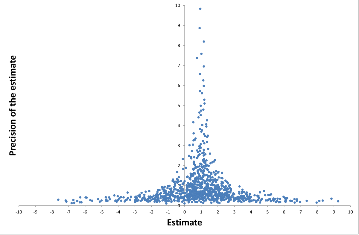
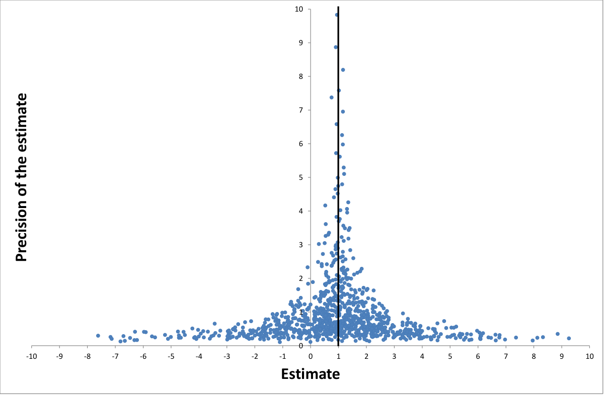
No bias, no correlation (?)

Researchers estimate

Earnings_j = γ Beauty_j + w_j.

They assume that γ̂/SE_γ̂ has a t-distribution.

→ estimates should not be correlated with standard errors (Card & Krueger, 1995)

Type I: Selection for the “correct sign.” Type II: Selection for statistical significance.

Simulation

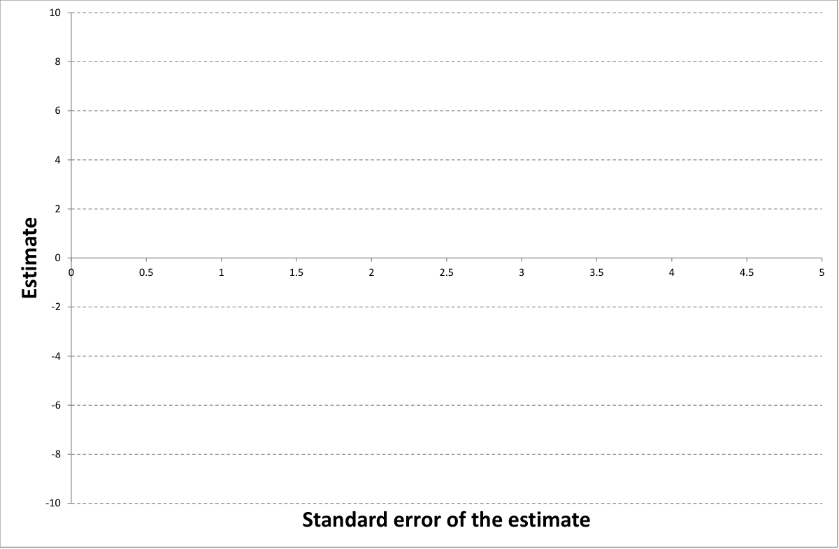
Simulation

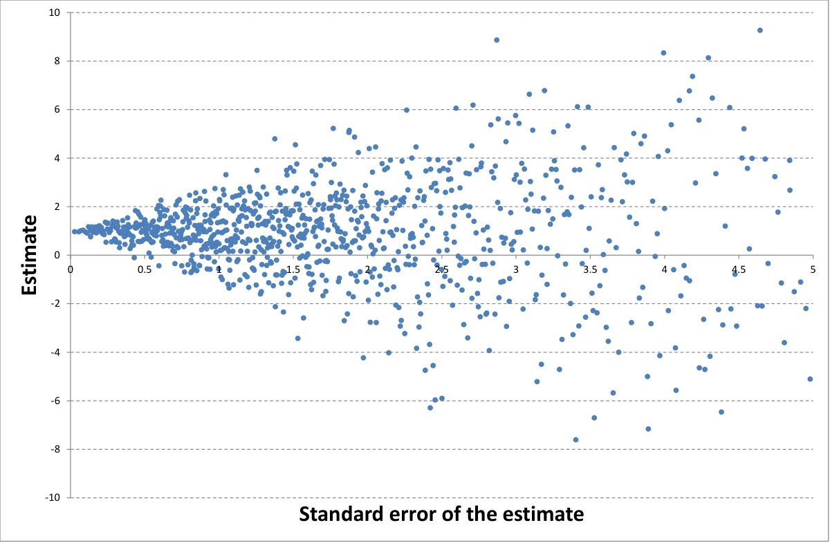
Simulation

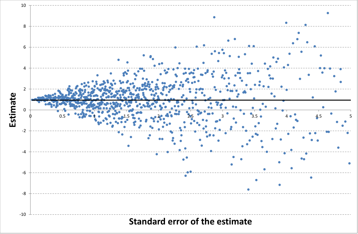
Simulation

Simulation

Simulation

Simulation

Simulation

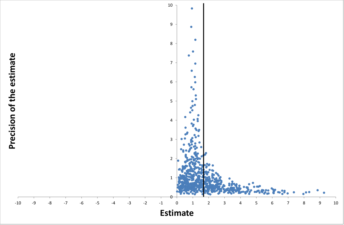
Simulation

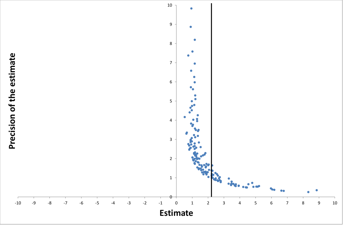
Funnel asymmetry test

In the absence of publication bias the funnel should be symmetrical: estimate_i = β [true effect] + β_0 SE_i [publication bias] + μ_i.

The equation is heteroscedastic. Weighted least squares yield

t_i = β_0 + β (1/SE_i) + ϑ_i. This is called the funnel asymmetry test, precision effect test (FAT-PET).

PEESE

Precision effect test with standard error (PEESE):

estimate_i = β [true effect] + β_0 SE^2_i [publication bias] + μ_i.

The equation is heteroscedastic. Weighted least squares yield

t_i = β_0 SE_i + β (1/SE_i) + ϑ_i.

WAAP (Ioannidis et al., 2017)

Weighted Average of Adequately Powered (WAAP) estimates.

• Focus on studies with adequate statistical power to reduce the impact of selective reporting.
• Combines results only from studies with at least 80% power.

Issues:

• Simple and robust.
• Need to estimate the true effect first and then compute power.

Stem-based correction technique (Furukawa, 2019)

Stem-based method:

• A non-parametric estimator that exploits the variance-bias trade-off.
• Focuses on the most precise estimates, referred to as the “stem” of the funnel plot.

Key features:

• Robust to various publication selection processes.
• Does not rely on specific distributional assumptions.

Application:

• Filters studies with the highest precision (lowest standard errors) to estimate the true effect.
• Reduces influence from noisier, potentially biased studies in the broader funnel plot.

Endogenous kink model (Bom & Rachinger, 2019)

Overview:

• Fits a piecewise linear model with a kink determined by the data.
• Identifies where publication selection is less likely to occur.

Key features:

• Endogenously estimates the cutoff based on standard errors.
• Often reduces bias and improves efficiency compared to traditional methods.

Application:

• Highlights genuine effects by focusing on less selective segments of the data.
• Effective in meta-analyses with substantial heterogeneity in study precision.

Selection model (Andrews & Kasy, 2019)

Overview:

• Models the selection process explicitly to address publication bias.
• Assumes researchers are more likely to publish statistically significant results.

Key features:

• Uses the likelihood of publication as a function of statistical significance.
• Adjusts estimates to reflect the missing studies.

Comparison to funnel-based models:

• Selection models are more rigorous but require stronger assumptions about the publication process.
• Funnel methods are simpler and more robust to model misspecification.

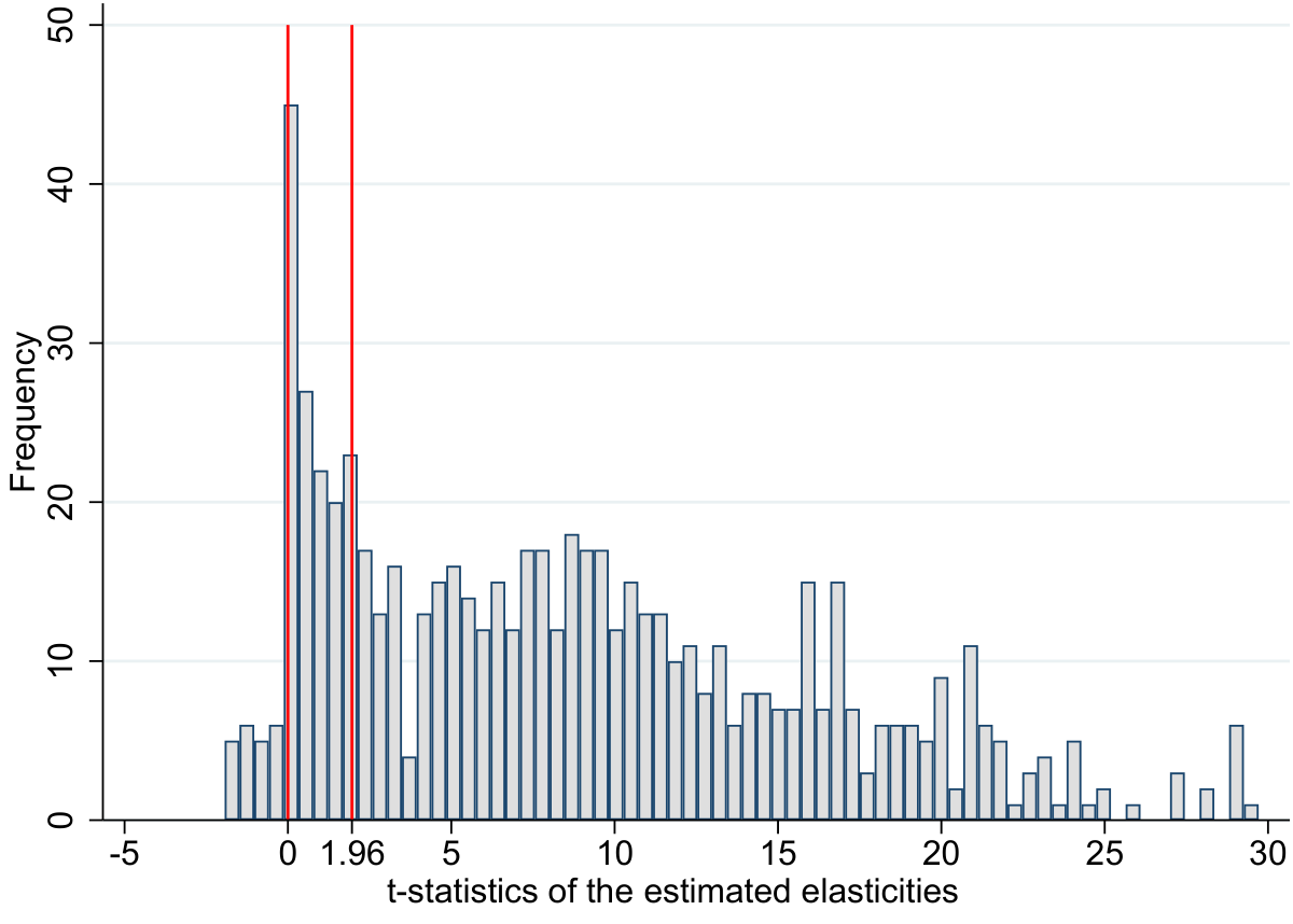
Example: labor supply elasticity

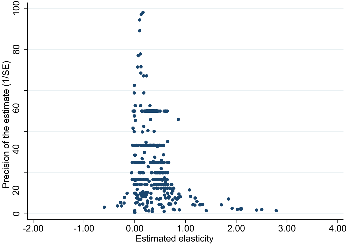
Results vary: RoBMA?

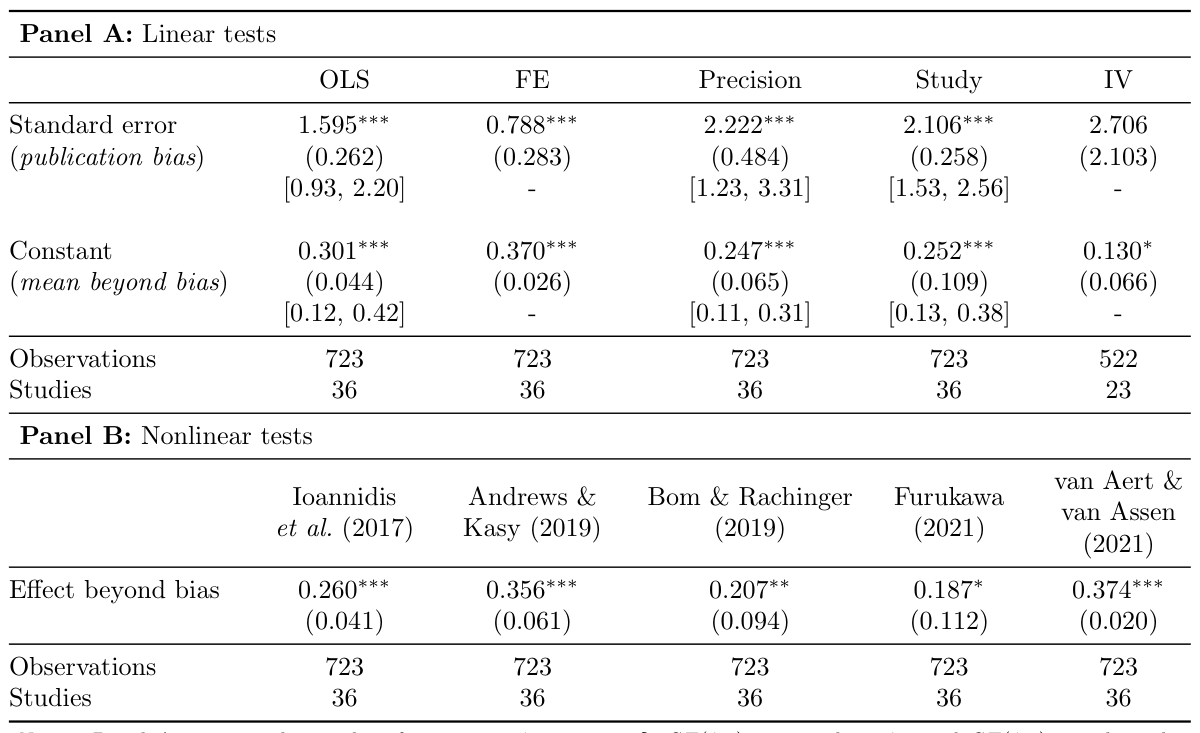
Bias caused by preference for positive estimates

Lecture 8: p-hacking

Recall publication bias

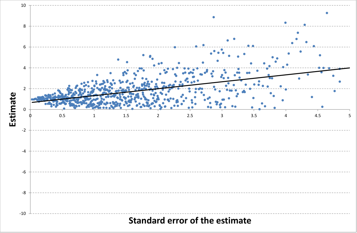
Recall publication bias

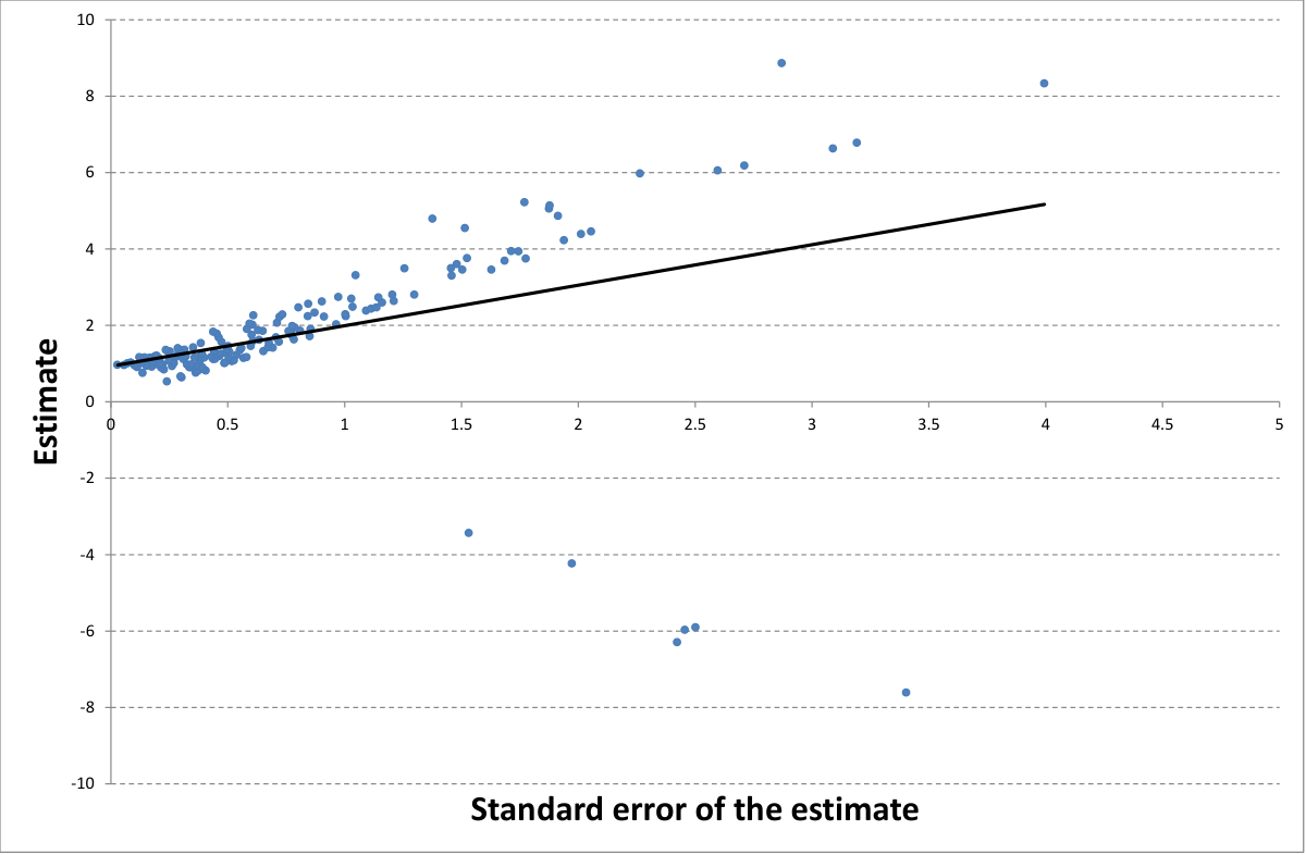
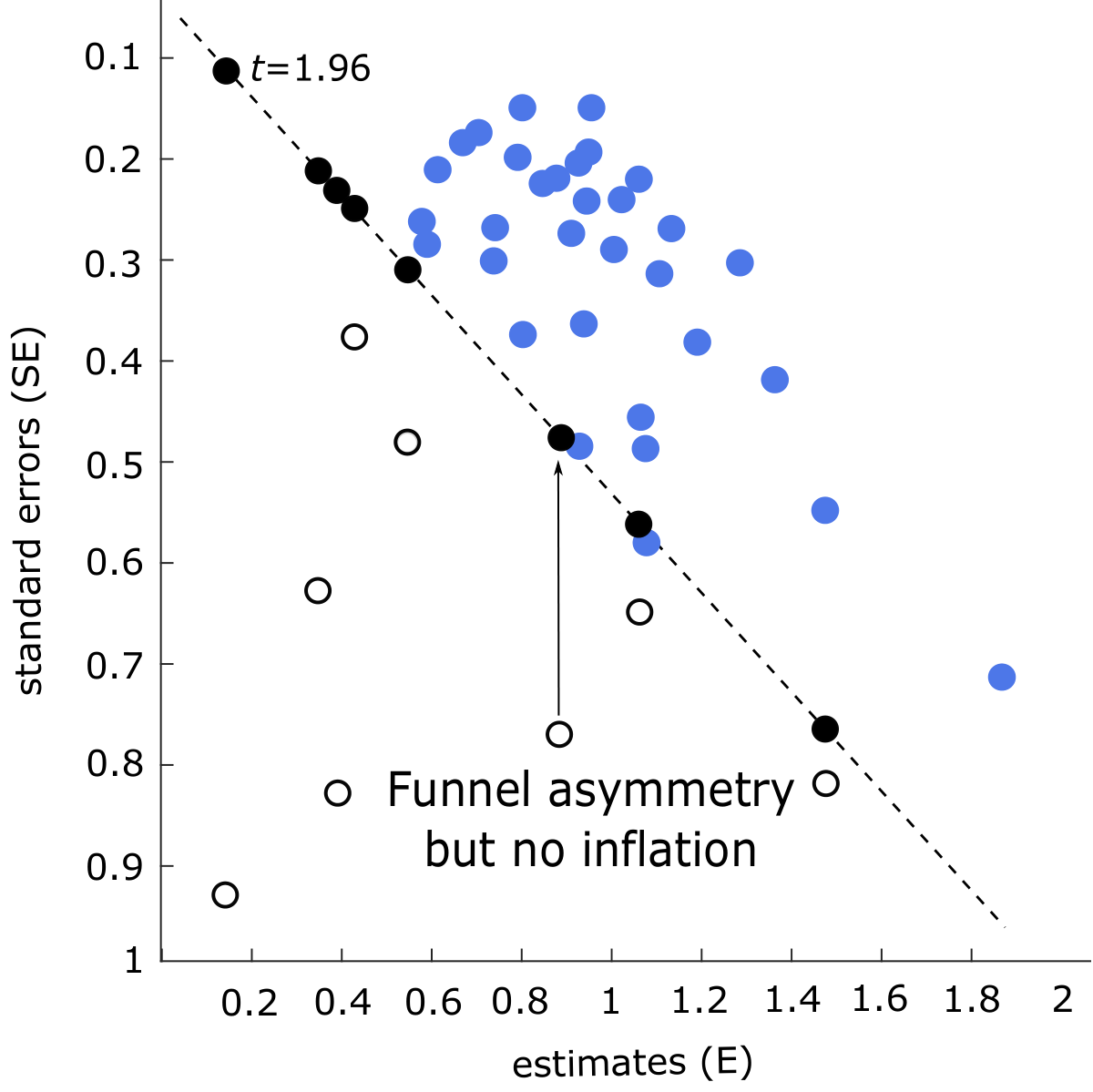
Key difference

• Publication bias: all estimates are individually unbiased
• The entire literature is biased because estimates are selectively reported
• If we know publication probabilities, we can recover the true effect (selection models)
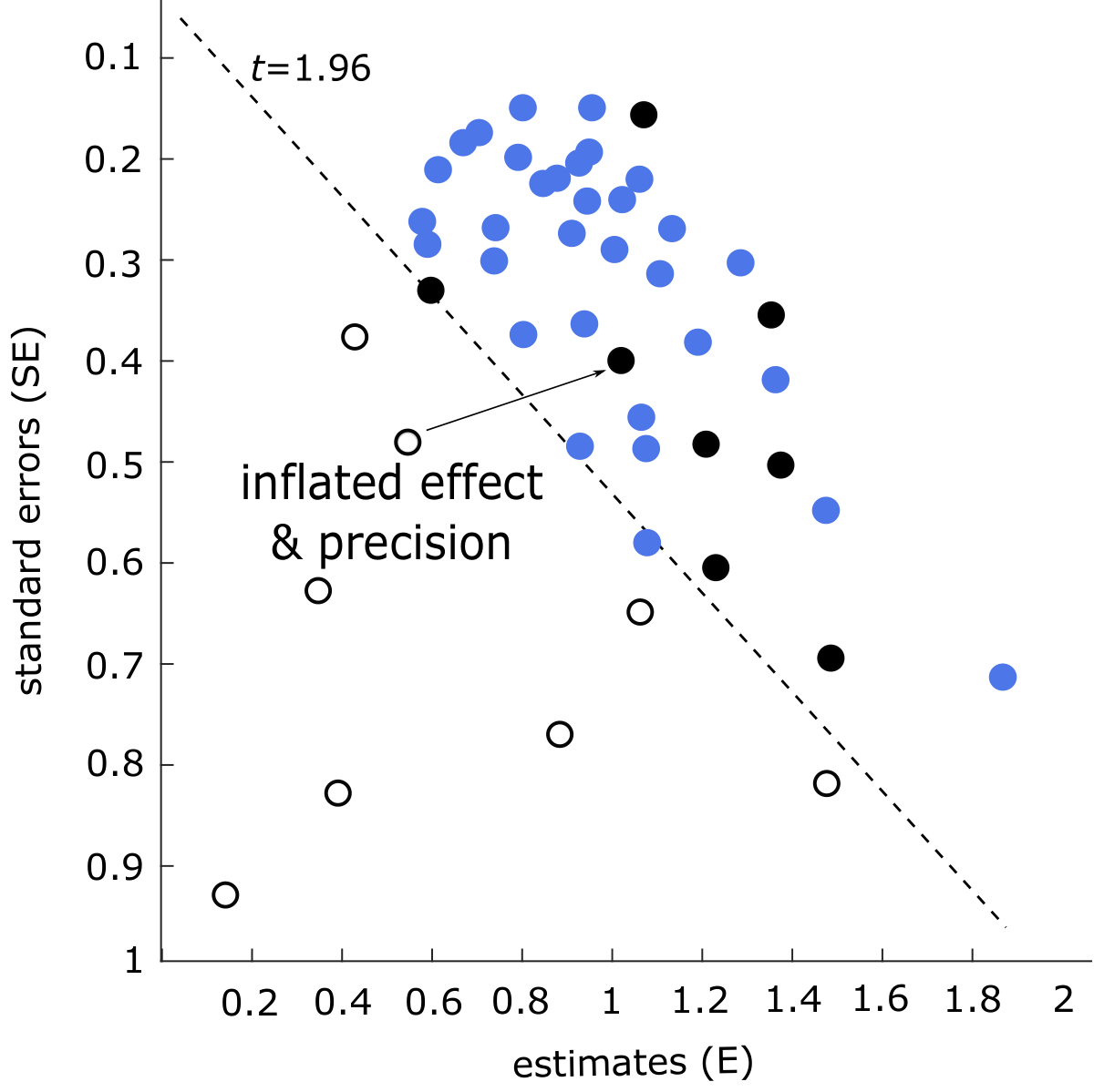
• P-hacking: individual estimates can be biased
• Classical selection models fail
• Funnel-based models can work (with adjustments)

Example: education premium

True model: Earnings_j = γ Education_j + δ Ability_j + v_j,

Omitted variable: Earnings_j = γ Education_j + w_j,

Proxy: Earnings_j = γ Education_j + ω IQ_j + x_j,

Instrument: Earnings_j = γ Education_j + z_j, Distance_j

Ability not observed.

Primary studies:

1. ignore ability → γ̂ too large, SE(γ̂) too small.
2. include a proxy → γ̂ smaller, SE(γ̂) larger.
3. quasi-experiment → γ̂ even smaller, SE(γ̂) even larger.

(With a diagram, in the PDF.)

Some estimates spuriously large & precise

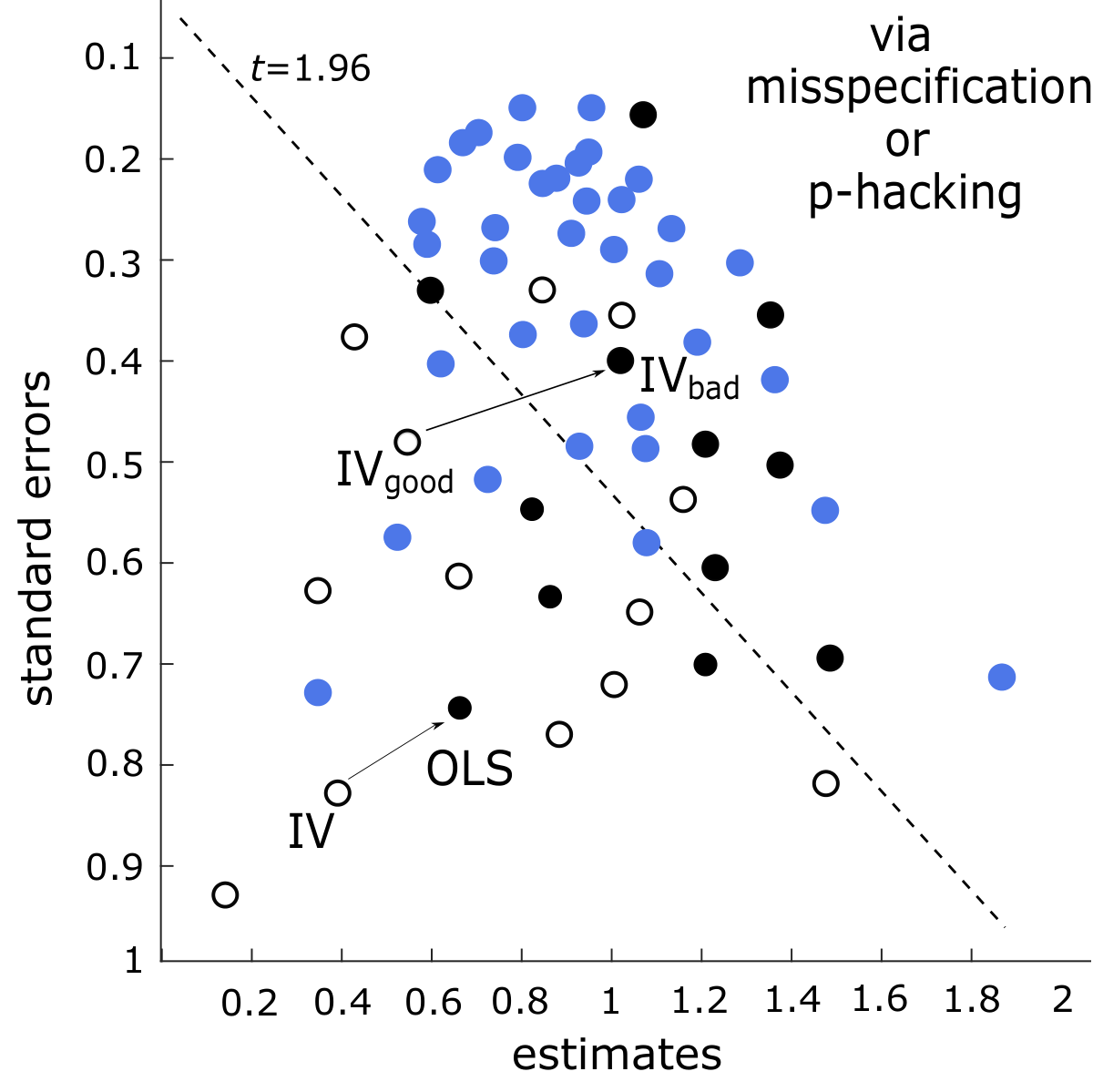
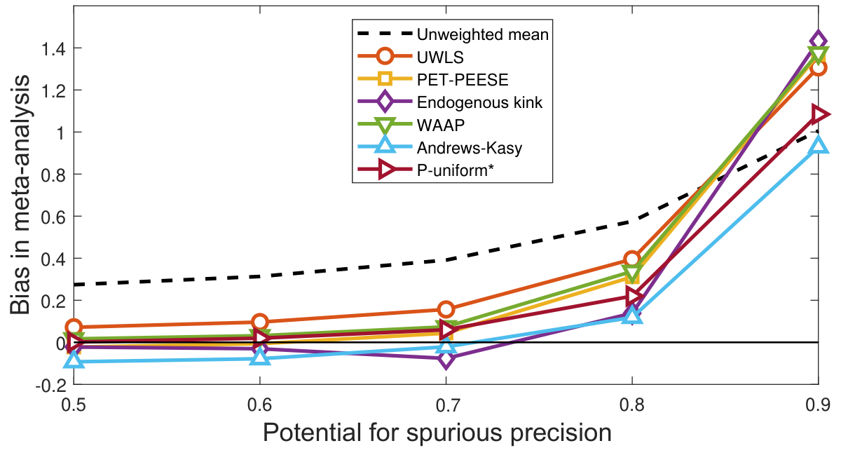
All estimators biased upwards

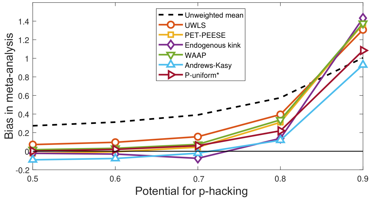
Example: Changing controls changes precision

Regression of test scores on class size

 | (1) | (2) | (3) | (4)
Small class (treatment) | 4.82 | 5.37 | 5.36 | 5.37
 | (2.19) | (1.26) | (1.21) | (1.19)
White/Asian |  |  | 8.35 | 8.44
 |  |  | (1.35) | (1.36)
Girl |  |  | 4.48 | 4.39
 |  |  | (0.63) | (0.63)
Free lunch |  |  | -13.15 | -13.07
 |  |  | (0.77) | (0.77)
White teacher |  |  |  | -0.57
 |  |  |  | (2.1)
Teacher experience |  |  |  | 0.26
 |  |  |  | (0.10)
Master's degree |  |  |  | -0.51
 |  |  |  | (1.06)
School intercepts | No | Yes | Yes | Yes
Sample | 5,861 | 5,861 | 5,861 | 5,861

Notes: Adapted from Krueger (1999). Dependent variable: test score percentile. Standard errors in parentheses.

Changing clustering changes precision

Regression of test scores on class size

 | Krueger (1999) | Replications using different computations of SE
 | (1) | (2) | (3) | (4) | (5) | (6)
 |  | Bootstrap of | Class | School | Huber-White | Plain vanilla
 |  | class clusters | clusters | clusters | SE | SE
Small class | 4.82 | 4.71 | 4.71 | 4.71 | 4.71 | 4.71
 | (2.19) | (2.00) | (1.88) | (1.38) | (0.79) | (0.76)
Sample | 5,861 | 5,743 | 5,743 | 5,743 | 5,743 | 5,743

Notes: Dependent variable: test score percentile. Standard errors (SE) in parentheses.

Available at meta-analysis.cz/class. (forthcoming in JOLE)

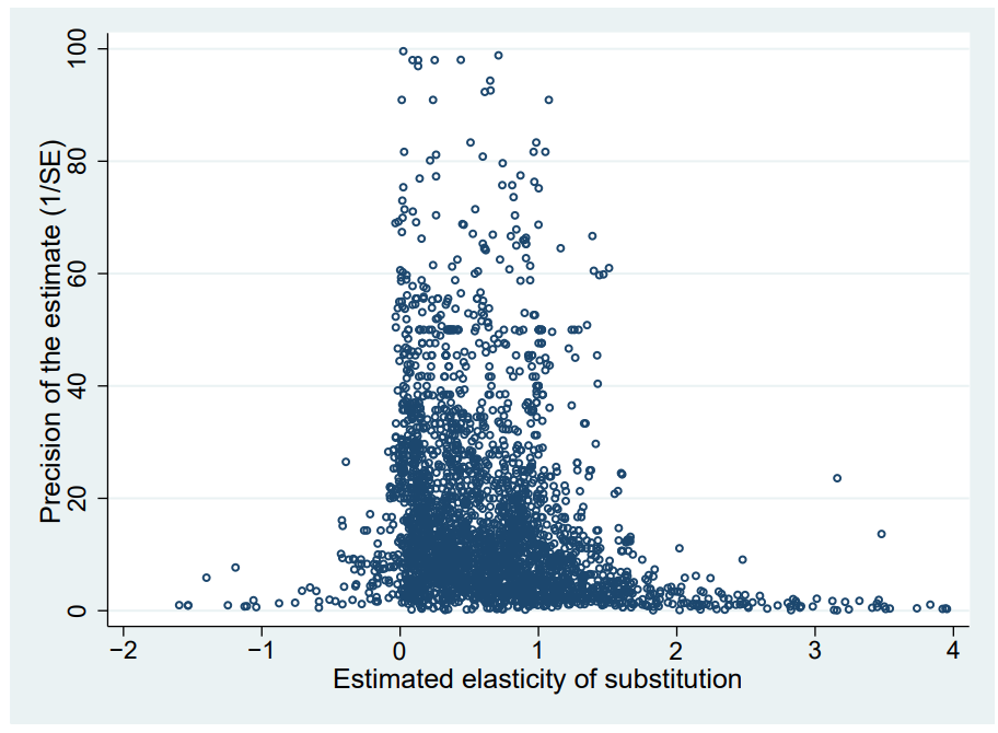
Funnel plot

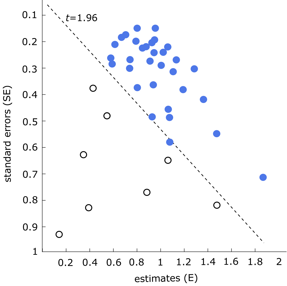
Publication bias

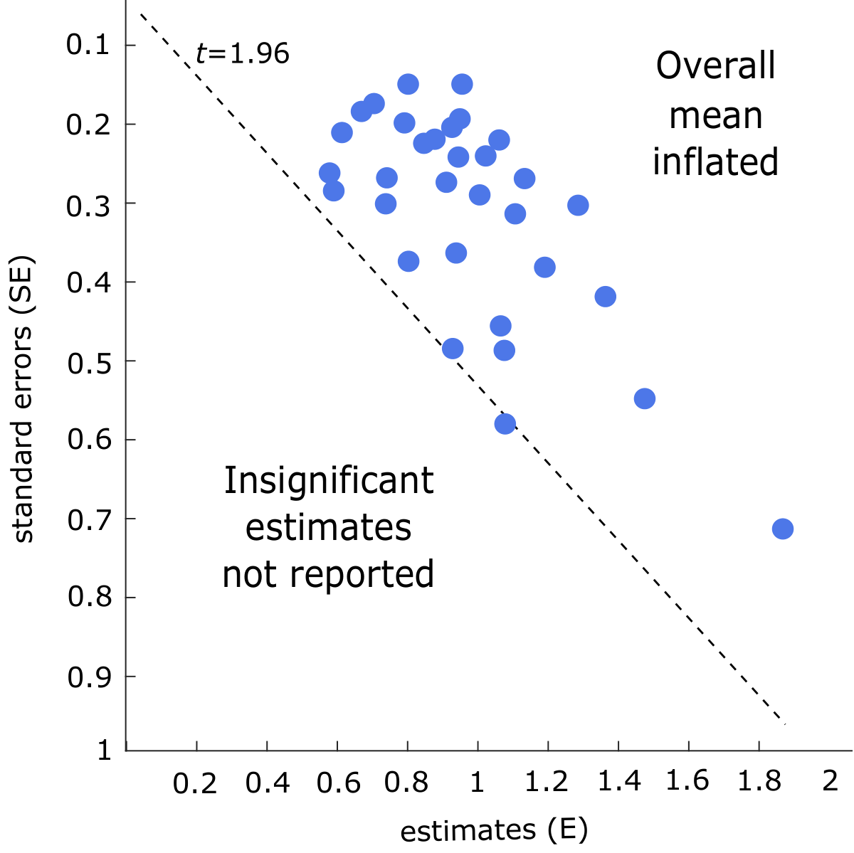
Conventional p-hacking

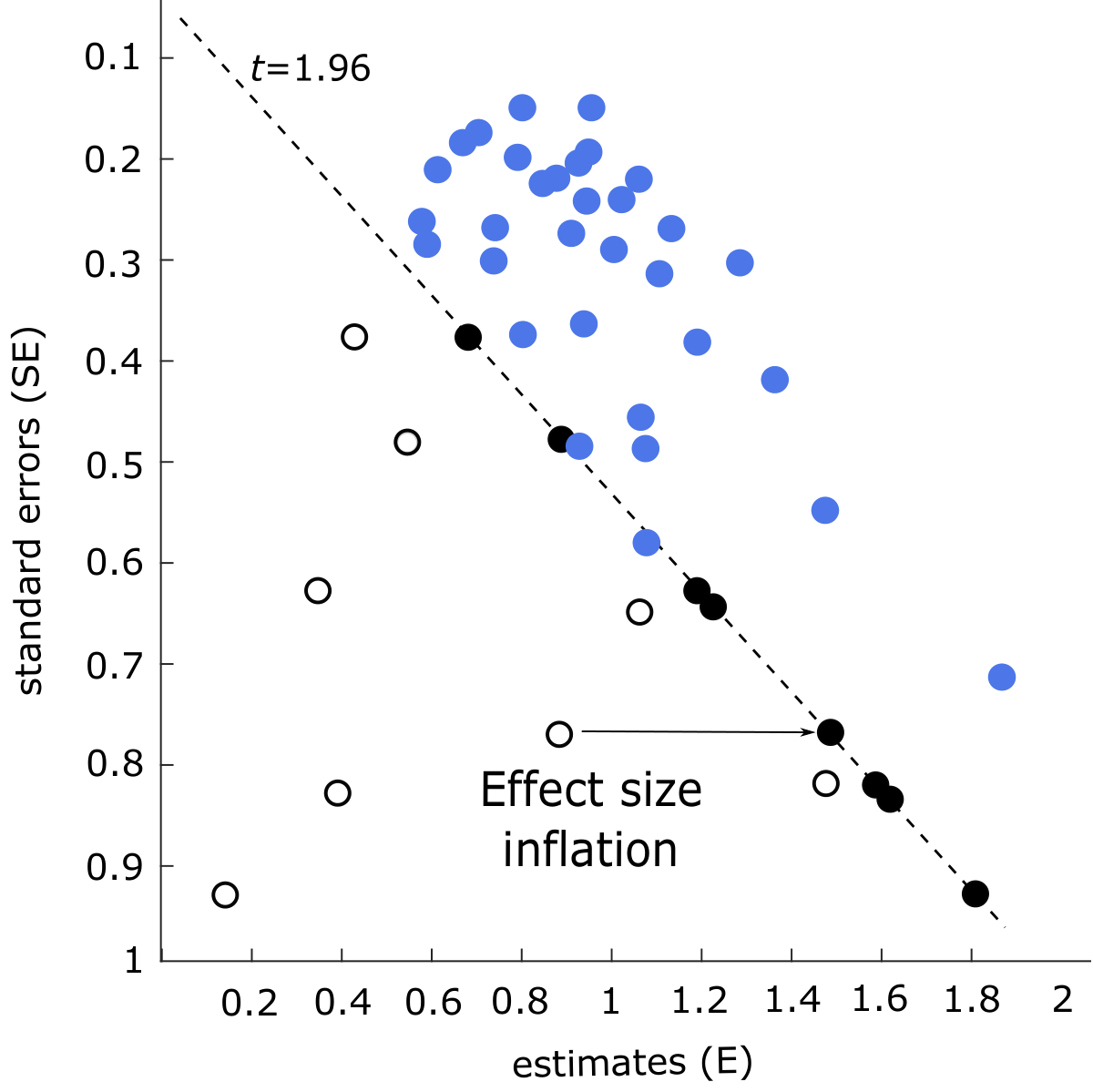
Spurious precision

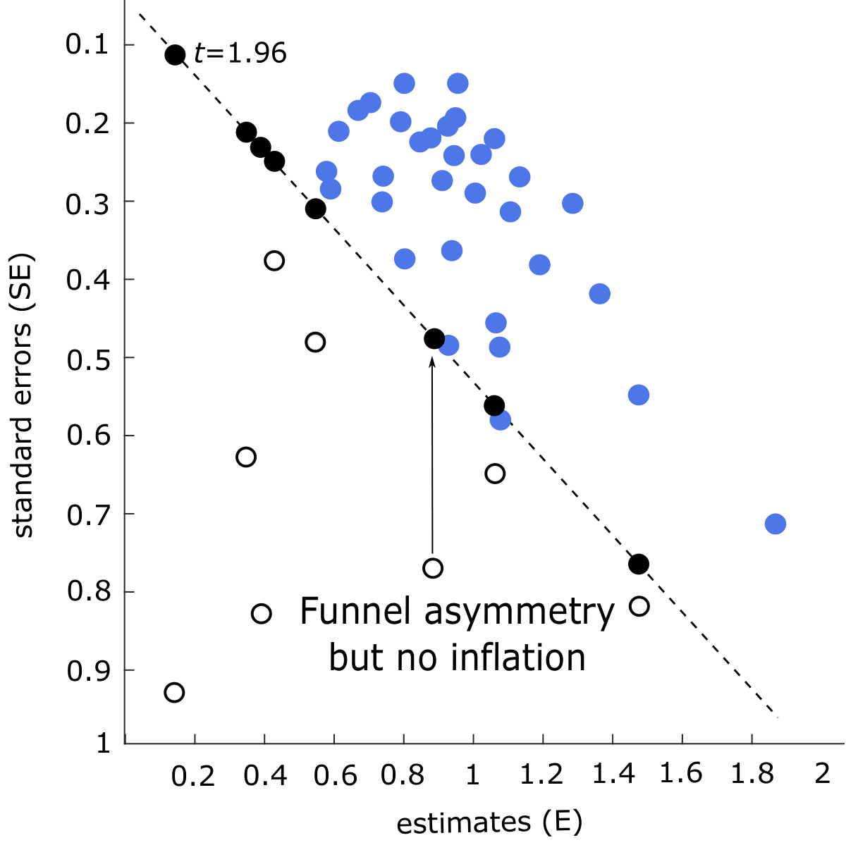
Key meta assumption broken

PEESE:

Ê_i = E_0 + β SE(Ê)^2_i + u_i,

corr(SE,u) ≠ 0 ⇒ β̂ and Ê_0 biased.

Natural solution: N instrumenting SE(Ê)_i^2 → MAIVE.

(With a diagram, in the PDF.)

Options for the meta-analyst

1. Use only quasi-experimental studies.
2. Include controls (dummies for OLS, DID, …). But in observational research we never know the true model!
3. Remove “bad” variation from SE → MAIVE.

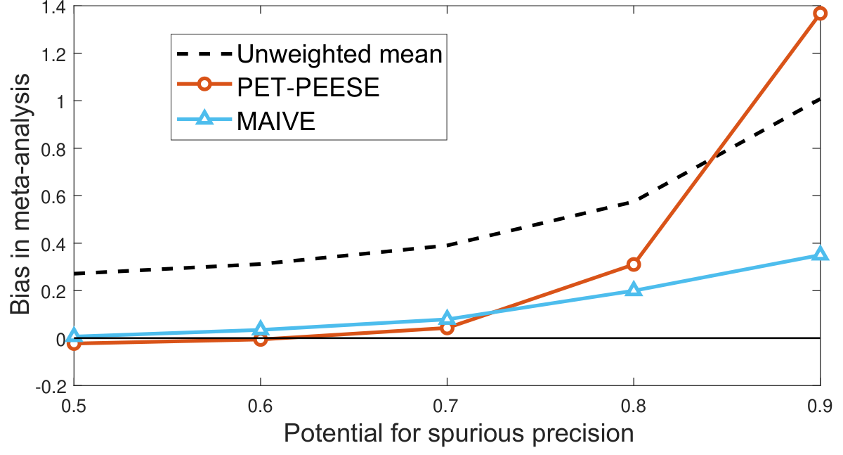
Meta-analysis instrumental variable estimator

MAIVE intuition: Ê_i = E_0 + β SE(Ê)^2_i + u_i, where the standard error, by definition, depends on 1/N_i.

MAIVE first stage: SE(Ê)^2_i = α_0 + α_1 (1/N_i) + π_i, where π_i stands for hacking or misspecifications.

MAIVE adjustment: SE(Ê)^2_(adj,i) = α̂_0 + α̂_1 (1/N_i). On the slide, π_i and its label, hacking or misspecifications, are struck out: the adjusted standard error keeps only the part explained by sample size.

• MAIVE + PEESE = classical IV.
• Can add controls in the 2nd stage.
• Plug MAIVE-adjusted SEs into other estimators.

(With a diagram, in the PDF.)

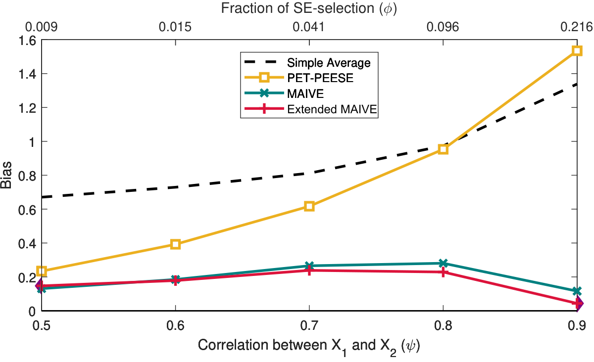
MAIVE alleviates the bias

Extended MAIVE

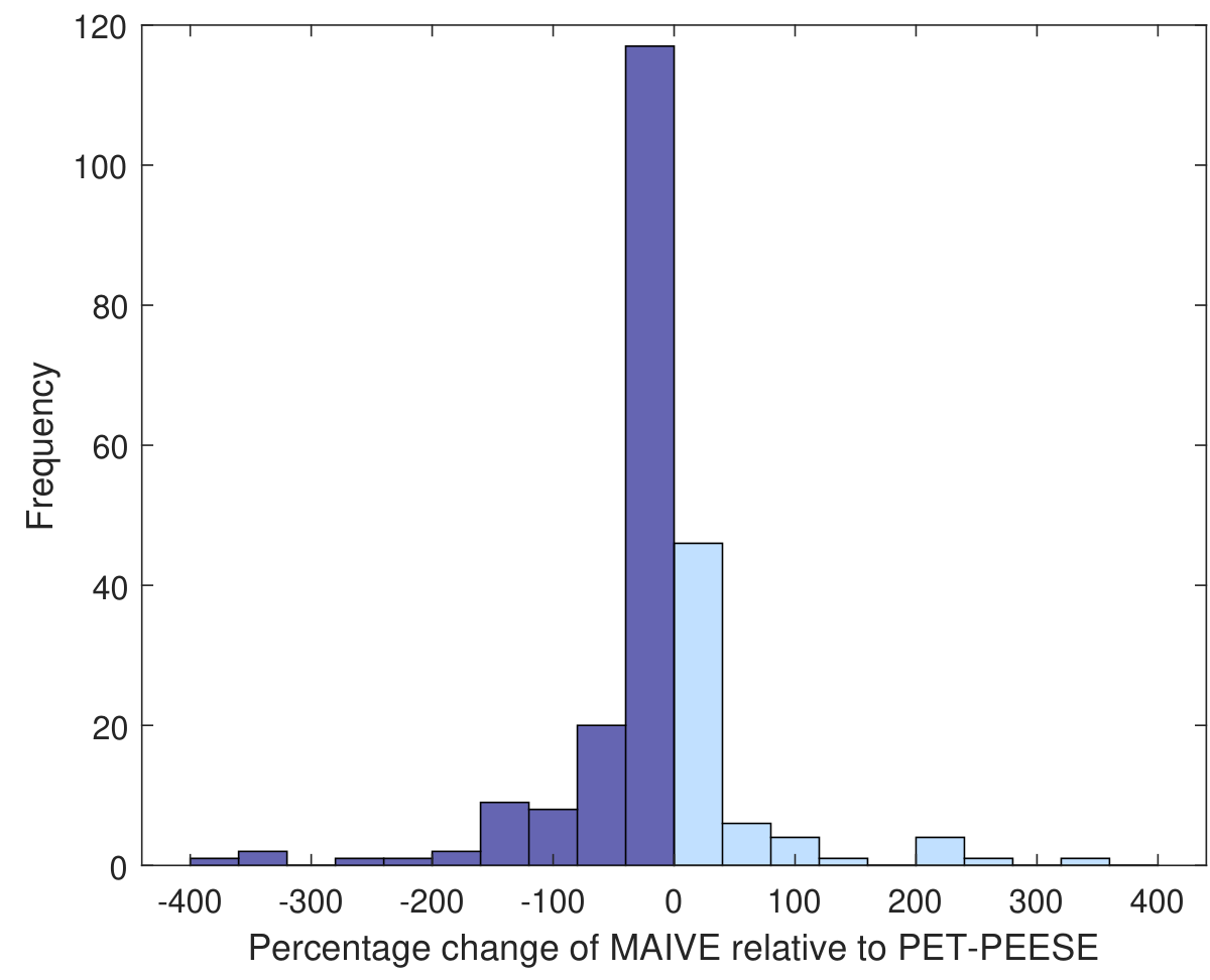
MAIVE reduces PET-PEESE in 70% of the cases

Practical issues

• Can methods or p-hacking influence both Ê and SE?
• Yes → MAIVE helps.
• No → MAIVE doesn't hurt much.

meta-analysis.cz/maive

Bonus: Maya Mathur's p-hacking correction

• Right-trunctated meta-analysis (RTMA, Mathur 2024, RSM)
• Assumption 1: insignificant estimates are NOT p-hacked
• Assumption 2: estimates are normally distributed
• Assumption 3: there are enough insignificant estimates published that we can recover the underlying distribution
• Bayesian techniques used for better convergence

Lecture 9: Heterogeneity

Identification of publication bias

PEESE:

Ê_i = E_0 + β SE(Ê)^2_i + u_i,

corr(SE,u) ≠ 0 ⇒ β̂ and Ê_0 biased.

Natural solution: N instrumenting SE(Ê)_i^2 → MAIVE.

Or add covariates!

(With a diagram, in the PDF.)

Classical heterogeneity measure

Common measure: estimate the relative heterogeneity of underlying effects (Higgins and Thompson, 2002)

I^2 ≡ (underlying variance of effects)/(observed variance of estimates) = τ^2/(τ^2 + v̄)

• I^2 = 0.75 ∼ 1.0 … “considerable heterogeneity” in medicine (Cochrane Review Guideline)
• I^2 ≃ 0.9 … common in economics meta-analyses (e.g., Vivalt, 2021)

Unresolved concern:

• no universally agreed criteria for “too much” heterogeneity
• undesirable pattern: with more precise studies, higher I^2

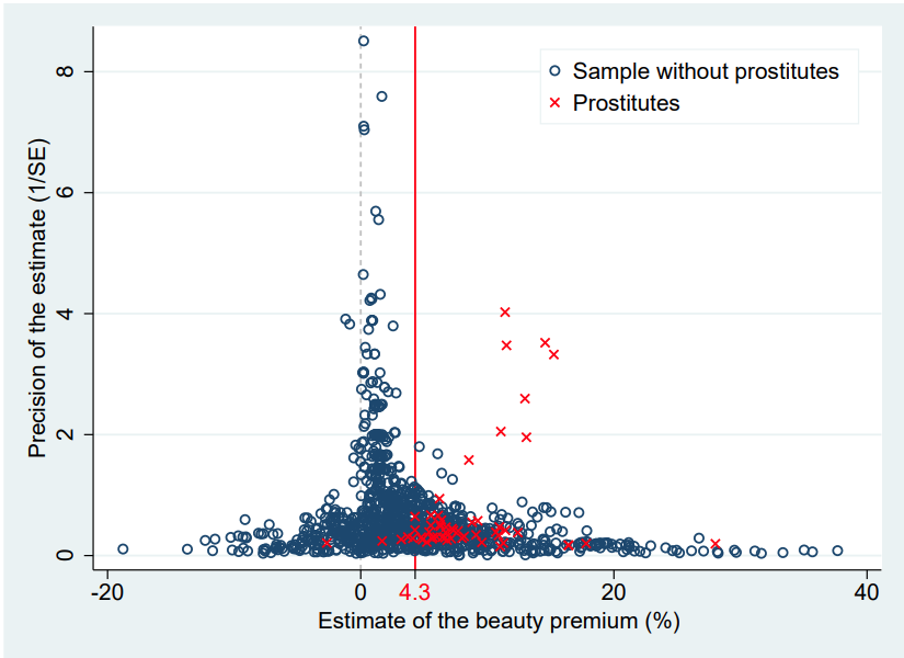
Guiding example: beauty and success

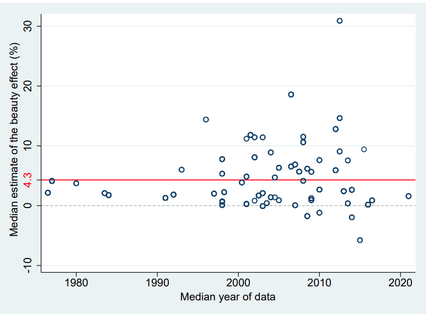
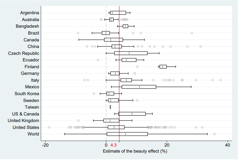
Heterogeneity both within and across

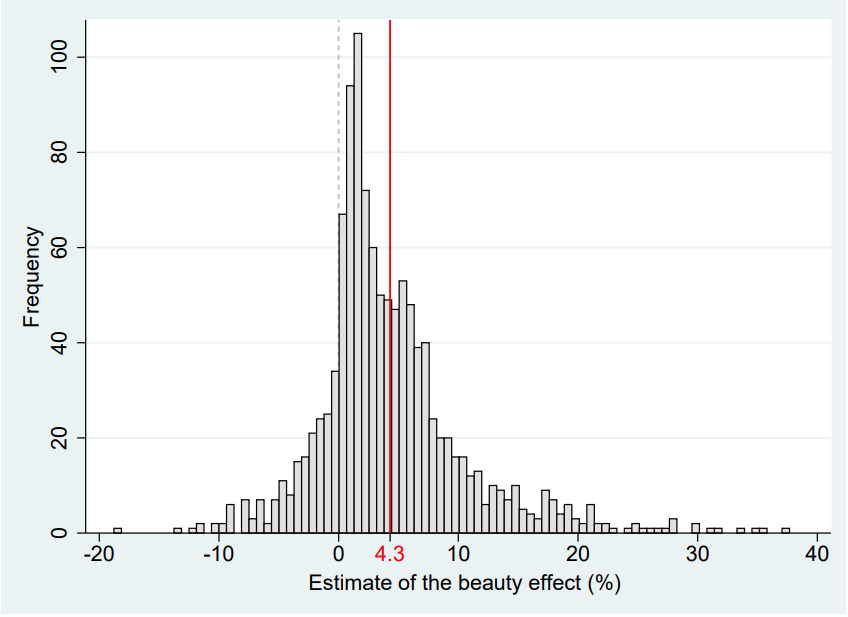
Wide dispersion

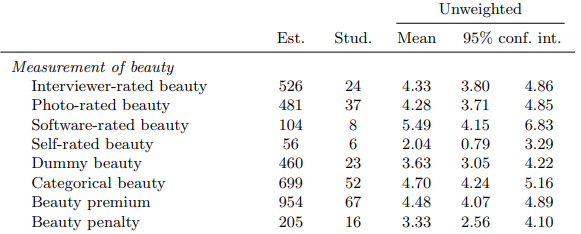
Measurement of beauty

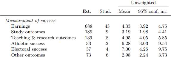
Measurement of success

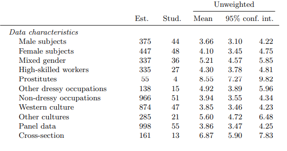
Data characteristics

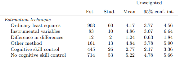
Estimation technique

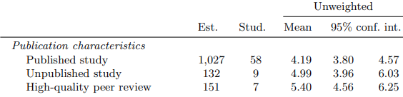
Publication characteristics

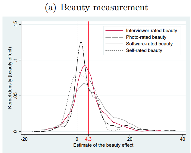
Beauty measurement doesn't matter

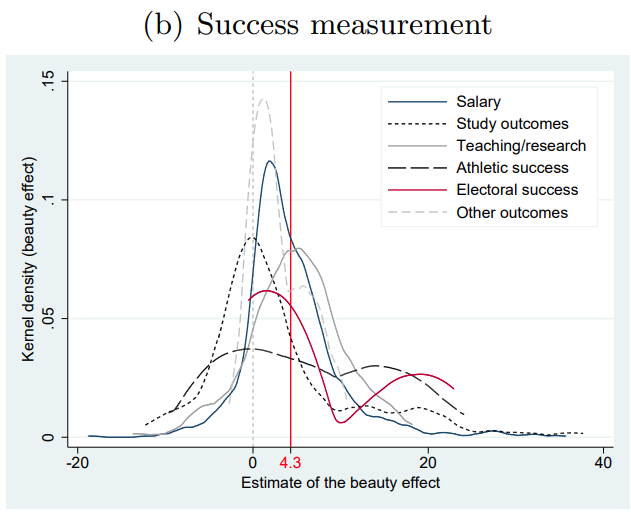
Success measurement doesn't matter

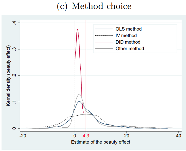
Method doesn't matter

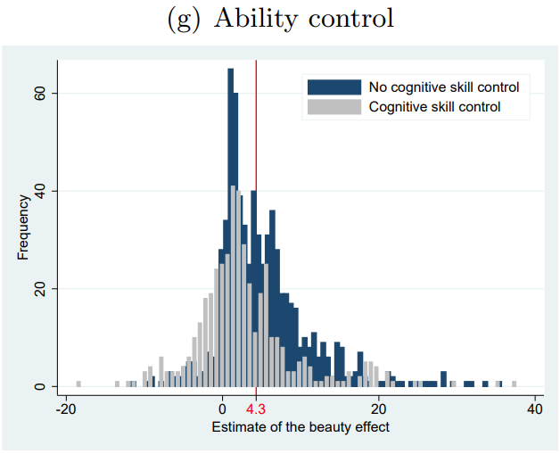
Ability control matters

Occupation matters

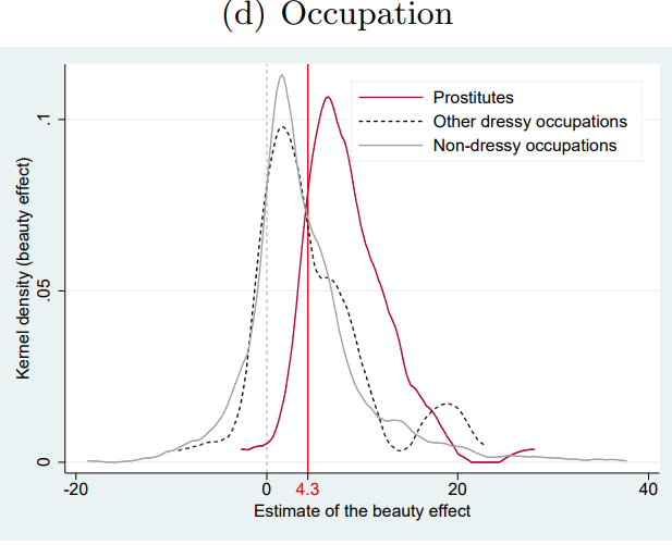
Sex workers stand apart

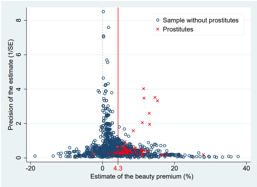
Option 1: subsamples

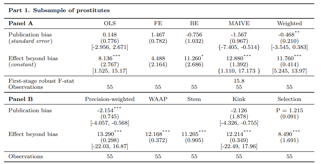
Option 1: subsamples

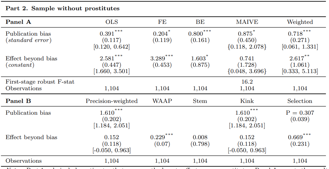
Option 1: subsamples

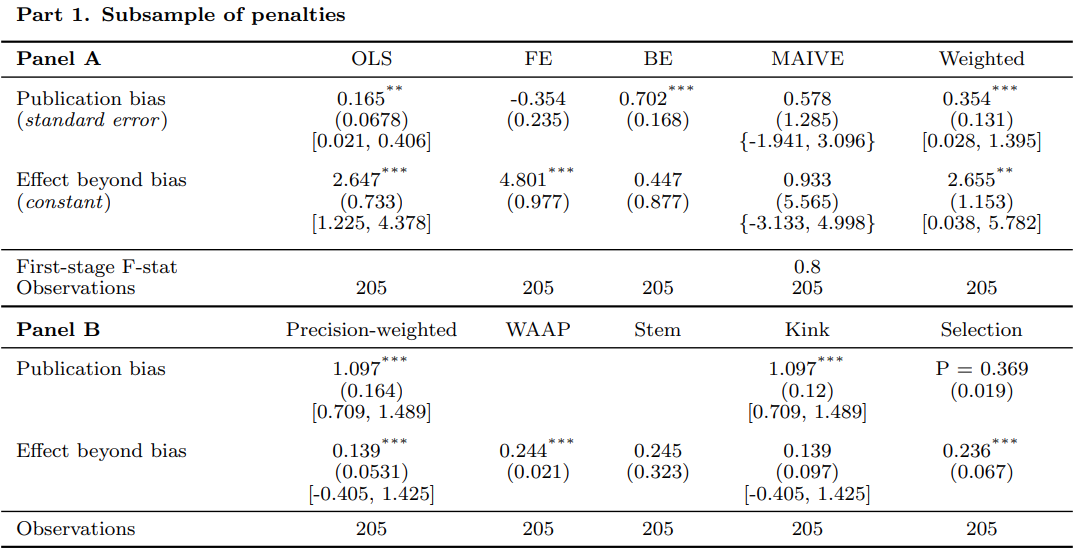
Option 1: subsamples

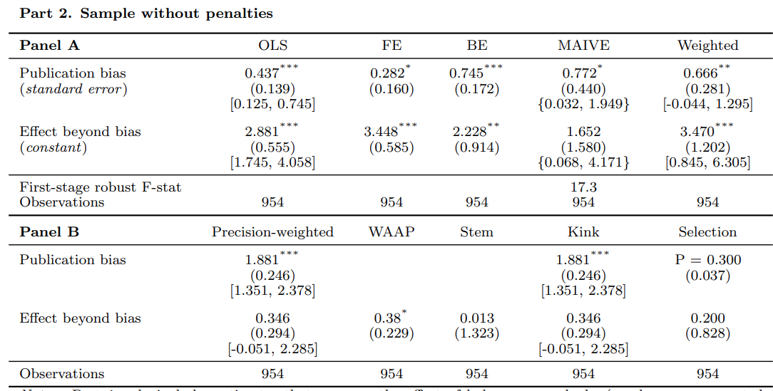
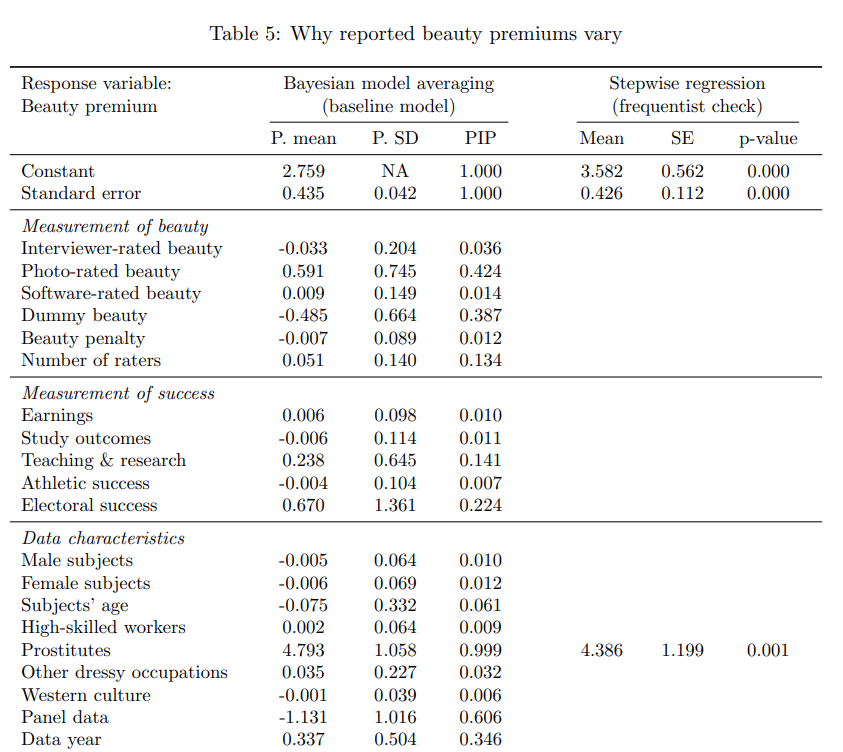
Option 2: Bayesian model averaging

• We want to regress estimates of the beauty effect on variables reflecting heterogeneity
• But too many variables; model uncertainty
• Solution: run regressions with different combinations of the variables
• Give more weight to those that fit the data well and are parsimonious

Option 2: Bayesian model averaging

• Model averaging can be frequentist but computationally difficult
• Intuition: run different combinations and weight by adjusted R^2 or information criteria
• In the Bayesian setting we can use the MCMC algorithm
• G-prior: all coefficients are zero. Weight? UIP = the prior has the same weight as one observation
• Model prior: uniform = all models have the same weight
• Dilution prior: models with collinearity get less weight

Model inclusion in BMA

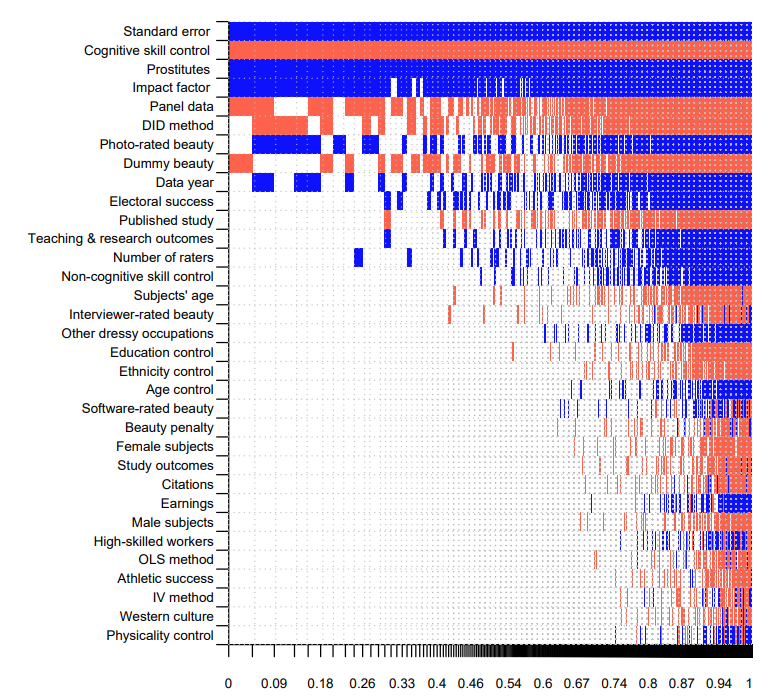
Posterior densities

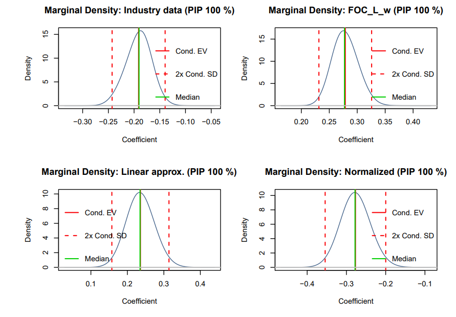
Regression results

Best practice (implied estimate)

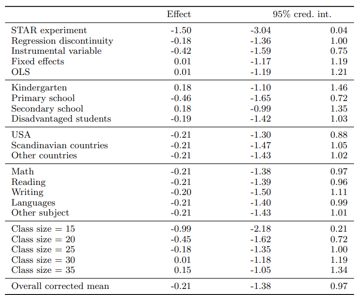
• From BMA results we know how estimates depend on study design
• Some study designs are better: identification, data, generally quality
• Select best practice based on the literature (quasi-experimental studies, etc.)
• Compute fitted values and confidence intervals (lincom command in Stata)

Best practice (class size effect)

Lecture 10: Meta-Research

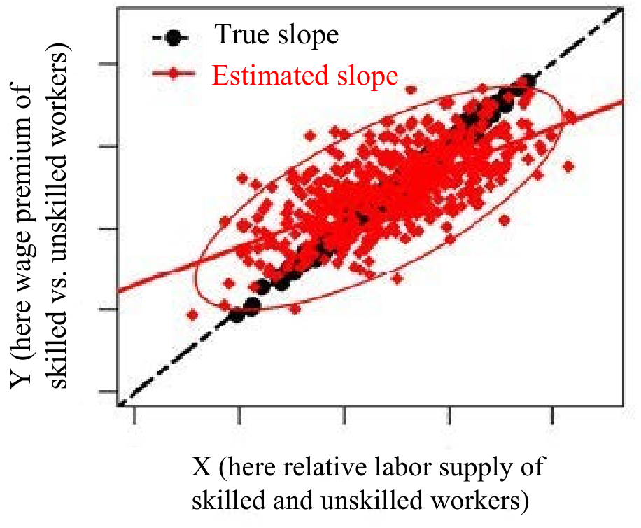
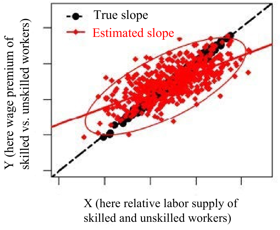
Example 1: Attenuation bias, aka regression dilution

Elasticity of skill substitution

Researchers estimate negative inverse elasticity: they regress skill premium on relative labor supply (not vice versa!)

• Measures substitutability between skilled (college) and unskilled (high school) workers
• Important for wage inequality, explaining cross-country differences in productivity, …
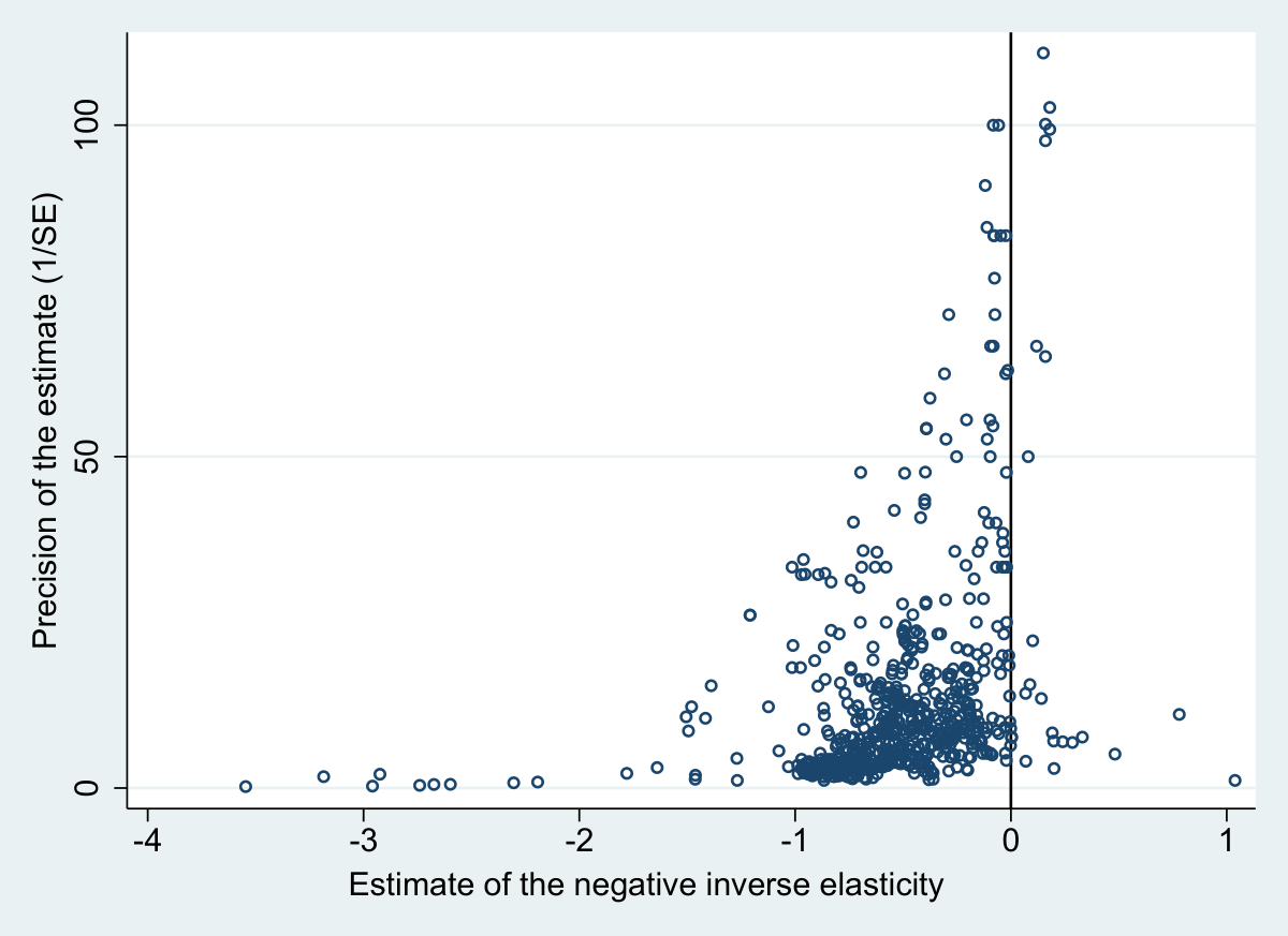
• 682 estimates from 77 studies, “consensus” elasticity = 1.5 (negative inverse = -0.67)

Three estimation frameworks

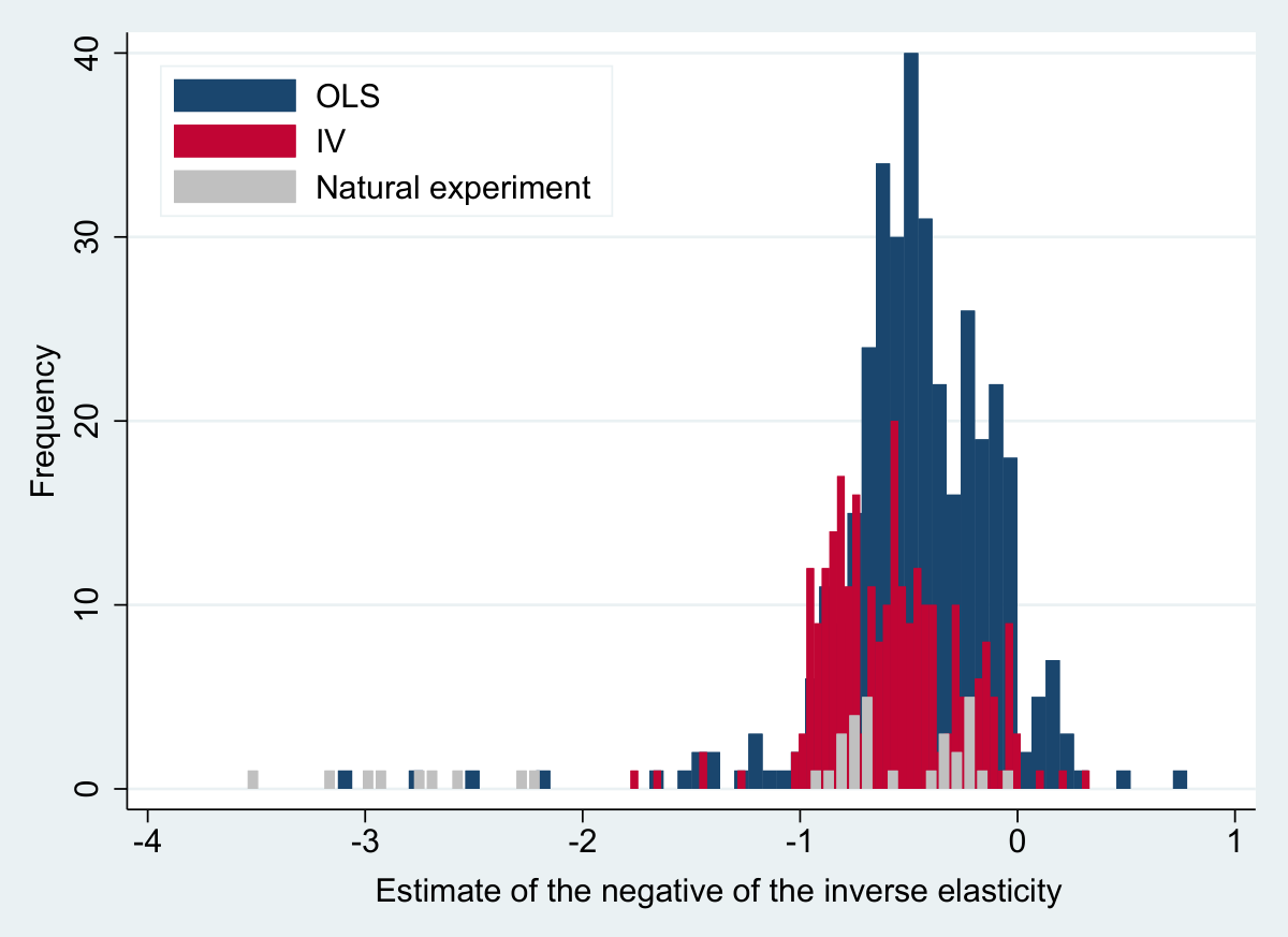
Strong publication bias (or p-hacking?)

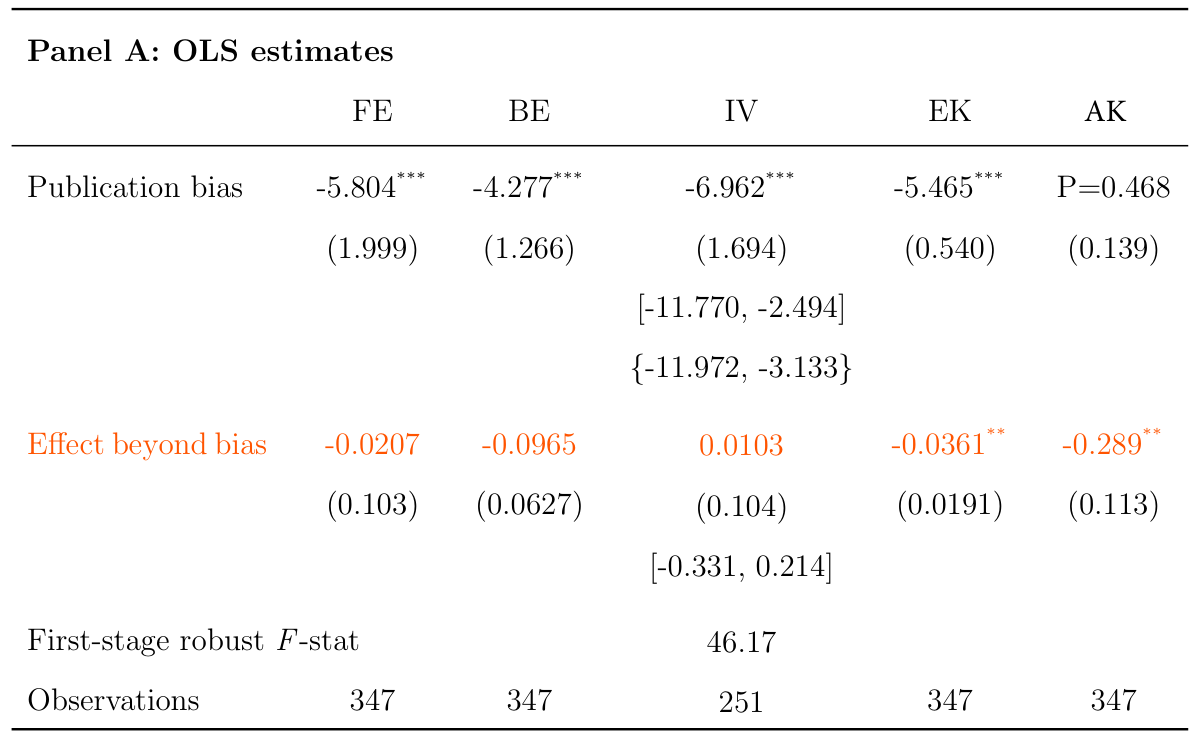
OLS: no effect (but attenuation & endogeneity biases)

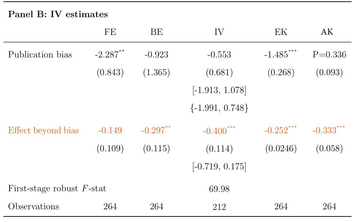
IV: strong effect (no biases beyond publication)

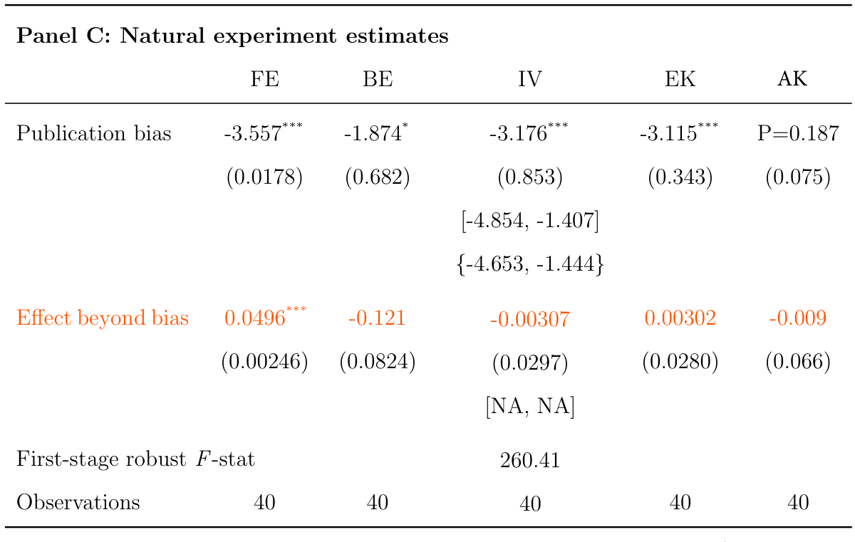
Natural experiments: no effect (but attenuation bias)

Publication bias > attenuation bias

• |IV| > |OLS| → attenuation or other endogeneity biases important
• OLS = Natural experiments → other endogeneity biases negligible
• |IV - OLS| measures attenuation bias, which is strong
• Uncorrected inverted elasticity = -0.67
• Inverted elasticity corrected for pub and attenuation bias (IV) = -0.25
• Pub bias dominates attenuation
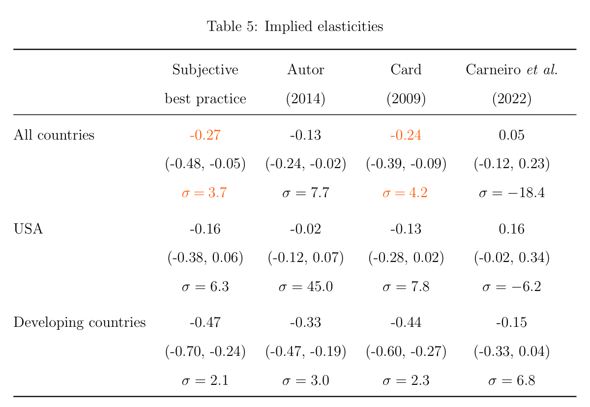
• Implied elasticity = 4

Assumptions of Andrews & Kasy not satisfied

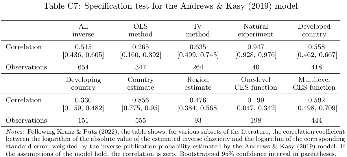
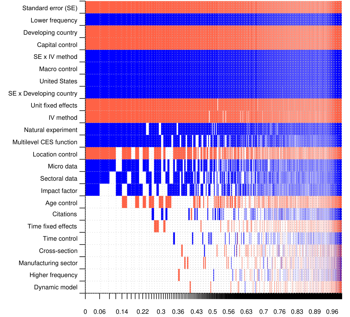
Model uncertainty; biases confirmed

Best practice estimate around 4

Results

1. Attenuation bias is important (|IV| > |OLS| = |natural experiments|).
2. Publication bias is more important (inverse elasticity: simple mean -0.67 ; corrected IV mean -0.25).
3. Implied elasticity around 4 (compared to consensus 1.5).

www.meta-analysis.cz/skill

Example 2: Too much heterogeneity?

Common measure: estimate the relative heterogeneity of underlying effects (Higgins and Thompson, 2002)

I^2 ≡ (underlying variance of effects)/(observed variance of estimates)

• I^2 = 0.75 ∼ 1.0 … “considerable heterogeneity” in medicine (Cochrane Review Guideline)
• I^2 ≃ 0.9 … common in economics meta-analyses (e.g., Vivalt, 2021)

Unresolved concern:

• no universally agreed criteria for “too much” heterogeneity
• undesirable pattern: with more precise studies, higher I^2

This Paper

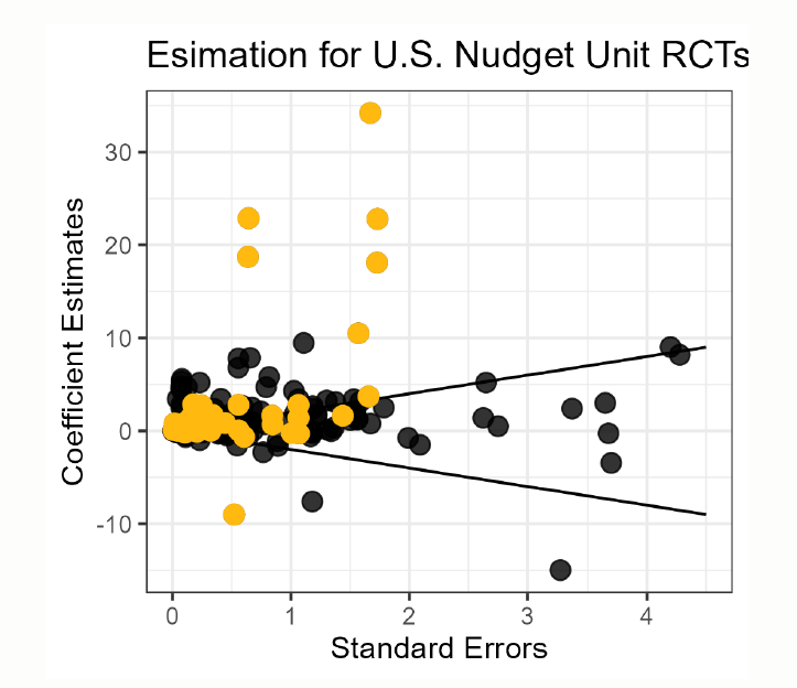
1. Propose a new test for external validity in meta-analysis:
   • Based on the tail index of the underlying distribution, without contamination by estimate precision.
   • Test whether the implied variance of underlying effect is infinite (i.e., too heterogeneous).
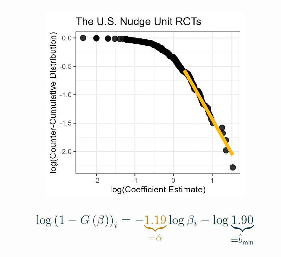
2. Show that the implied variance is infinite in meta-analysis of 126 nudge RCTs (DellaVigna and Linos, 2020):
   • Nudge: “choice architecture that alters people's behavior in a predictable way without forbidding any options or significantly changing their economic incentives.” (Thaler and Sunstein, 2008)
   • The possibility of infinite variance can be important in real-world applications.

Test of Infinite Variance

Pareto tail: F(b) = 1 - Cb^(-α), b > b_min and C > 0

• e.g. earthquakes, word frequency, city size, wealth distribution
• If α < 2, then Var(b) = ∞ because ∫_b_min^∞ b^2 f(b) db ∝ ∫_b_min^∞ b^2 b^(-3) db = ∫_b_min^∞ b^(-1) db = log b |_b_min^∞ = ∞

Tail Index Test of External Validity:

• Criteria 1: if α̂ > 2, then pass the test
• Criteria 2: if P(α̂ ≤ 2) < p, then pass the test

Estimation Methods (i) Inner Problem of Tail Index

Following Hill (1975), use Maximum Likelihood Estimation for α̂_MLE: given b_min, α̂_MLE = arg max_α Σ_(i=1)^n ln l ( α | β_i, SE_i, b_min ), where l ( α | β_i, SE_i, b_min ) ≡ ∫_θ_min^∞ (φ ( (β_i - θ)/SE_i ))/(1 - Φ ( (b_min - θ)/SE_i )) α b_min^α b^(-(α + 1)) db.

• Numerical integration

Estimation Methods (ii) Outer Problem of Cut-off

Following Clauset et al. (2006), use the goodness-of-fit metric to choose b^*_min: b^*_min ∈ arg min_b_min K̃S (b_min | α̂_MLE), where the reweighted Kolmogorov-Smirnov statistic is K̃S (b_min | α̂_MLE) ≡ sup_β (|G(β | β ≥ b_min) - Ĝ(β | ·)|)/(√(Ĝ(β | ·) [1 - Ĝ(β | ·)])), and the estimated distribution is Ĝ(β | α̂_MLE, β ≥ b_min) and the empirical distribution is G(β | β ≥ b_min).

Nudges

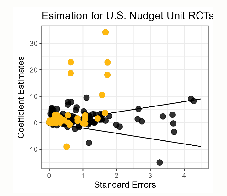
Nudges

Summary

1. Proposed the concept of “infinite variance” as representing the persistent criticism that “too much” heterogeneity underlies the overall mean estimate.
2. Developed an estimation method by extending the maximum likelihood estimation and goodness-of-fit statistics commonly used in tail estimation.
3. Applied the estimation method and its implied test to show that the influential nudge meta-analysis exhibits the infinite variance.

Lecture 11: Limitations of Meta-Analysis

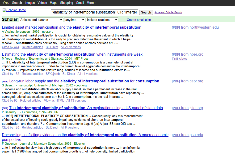
Scholar search replicability

Universal coverage

Measurement error

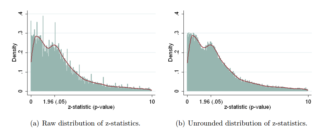
Rounding

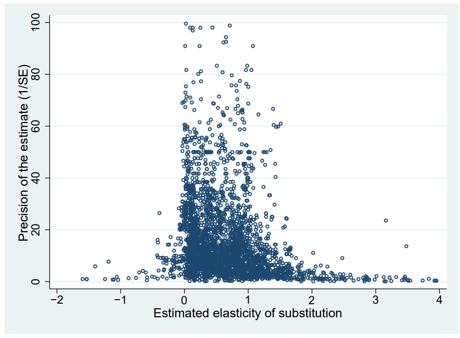
Outliers

Too much heterogeneity

Too much heterogeneity

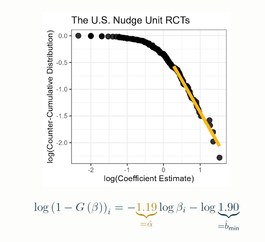
Too much heterogeneity

Identification

Omitted variables

Attenuation bias

Partial correlations

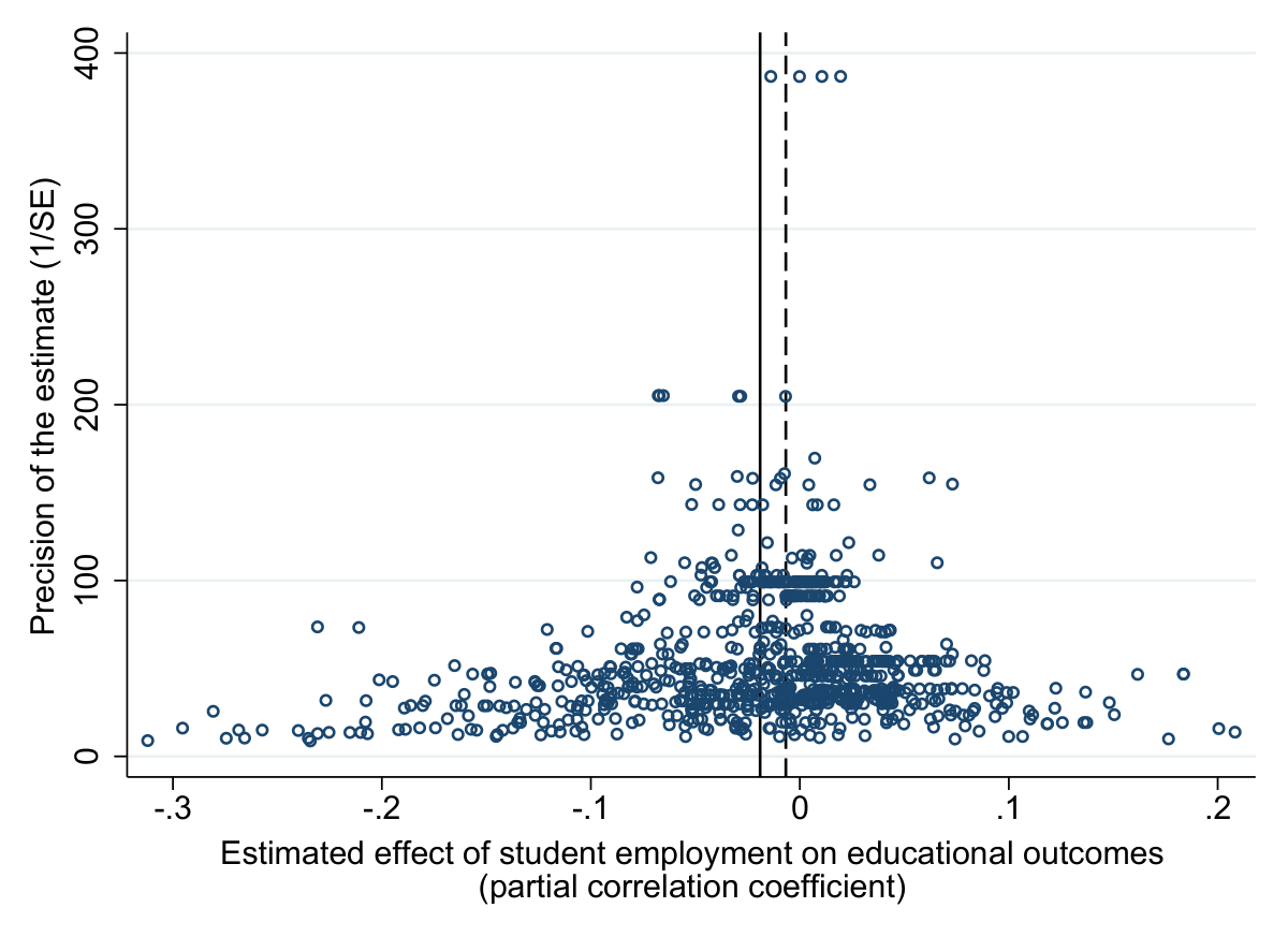
Partial correlations

r_p = t/(√(t^2 + df)),

S_1^2 = ((1 - r_p^2)^2)/df,

S_2^2 = (1 - r_p^2)/df.

Inverse coefficients

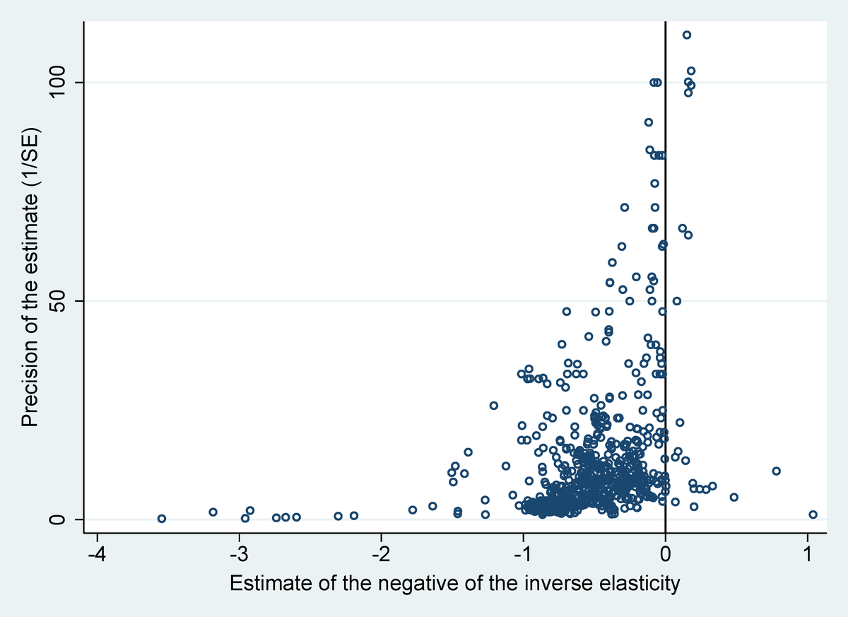
Delta method

Based on Taylor series expansion. Basic formula:

Var(Y) = Var(f(X)) ≈ [f'(μ_X)]^2 Var(X).

Example: Suppose Y = X^2. Then f(x) = x^2 and f'(x) = 2x, so that: Var(Y) ≈ [2μ_X]^2 Var(X) = 4μ_X^2σ_X^2.

Example: Suppose Y = 1/X. Then f(x) = 1/x and f'(x) = -1/x^2, so that: Var(Y) ≈ [(-1)/μ_X^2]^2 Var(X) = σ_X^2/μ_X^4.

Tests disagree

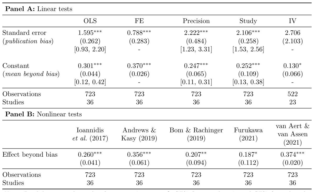
P-hacking

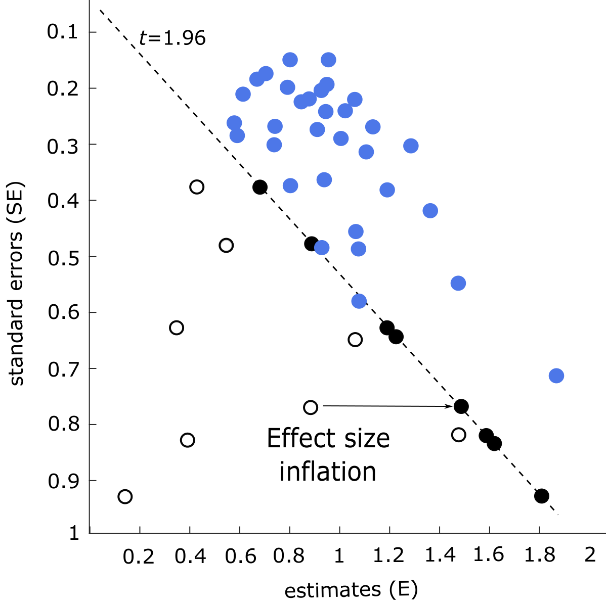
P-hacking

P-hacking

Bias in meta estimators