Motivation

Meta important for research, policy, practice

Research experience:

• Affiliate at the Meta-Research Innovation Center, Stanford
• Panel member at ERC Advanced
• Convener of Meta-Analysis in Economics Network
• Meta-Analysis Editor at the Journal of Economic Surveys
• MAIVE method (Nature Communications)
• Over 50 metas published, e.g. REStat, JEEA, JOLE, JIE…

Policy experience:

• Former Advisor to the Board, Czech National Bank
• Former member of the Czech National Economic Council
• Affiliate at the Centre for Economic Policy Research, London

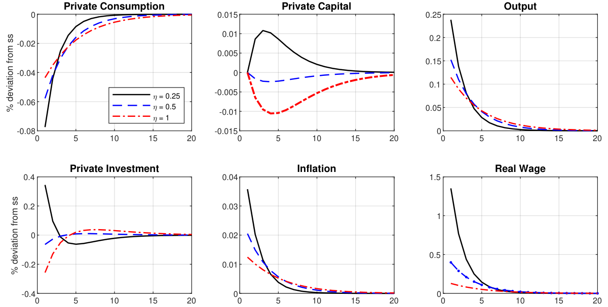
What happens if the government spends more?

Labor supply elasticity is key (but how to calibrate it?): Details: Elminejad et al. (2023, Review of Economic Dynamics)

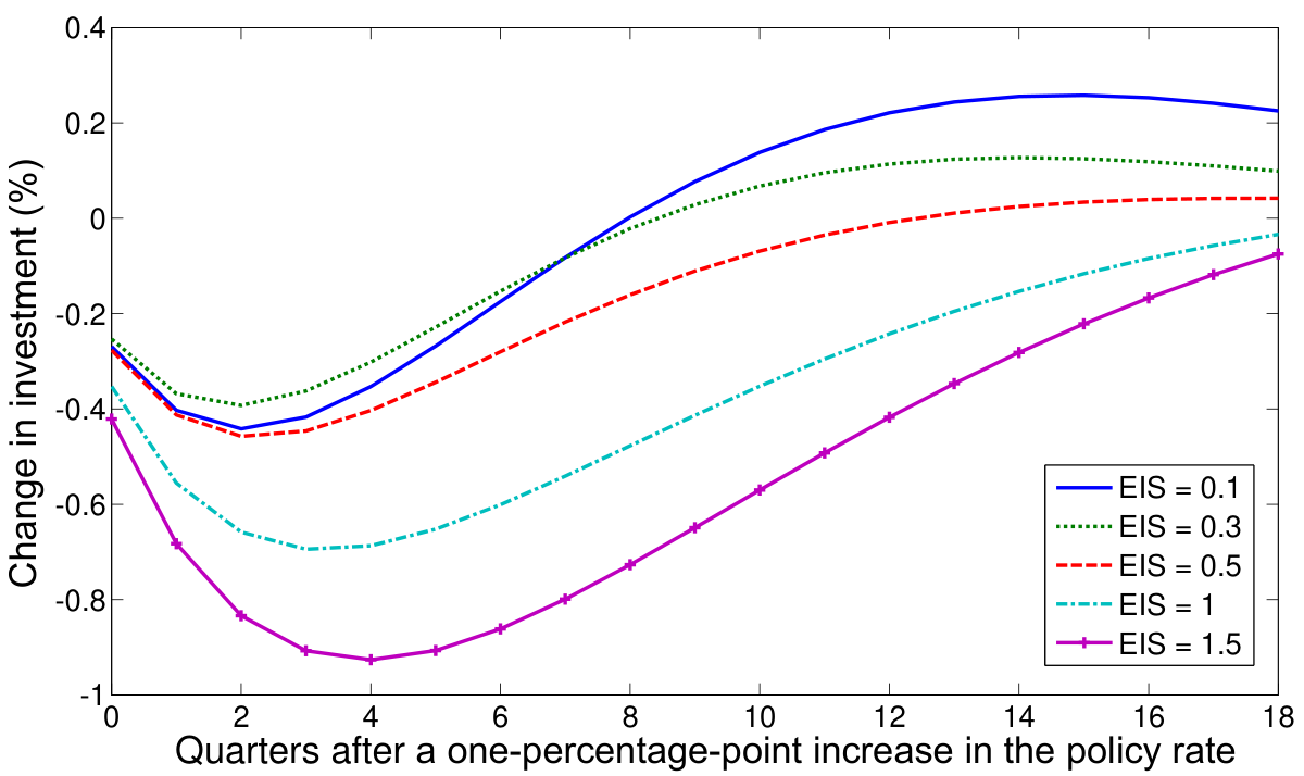
What happens if the central bank raises the rate?

Details: Havranek et al. (2015, Journal of International Econ)

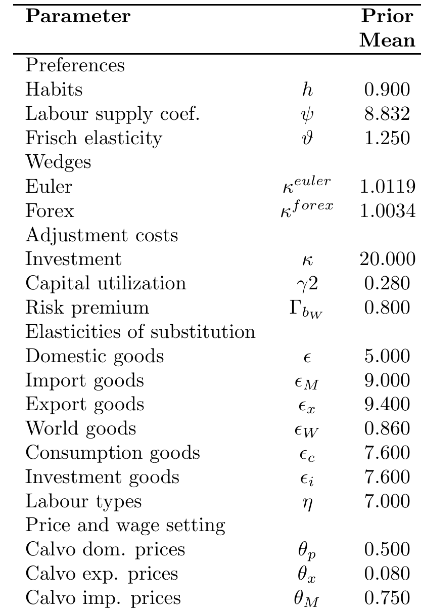
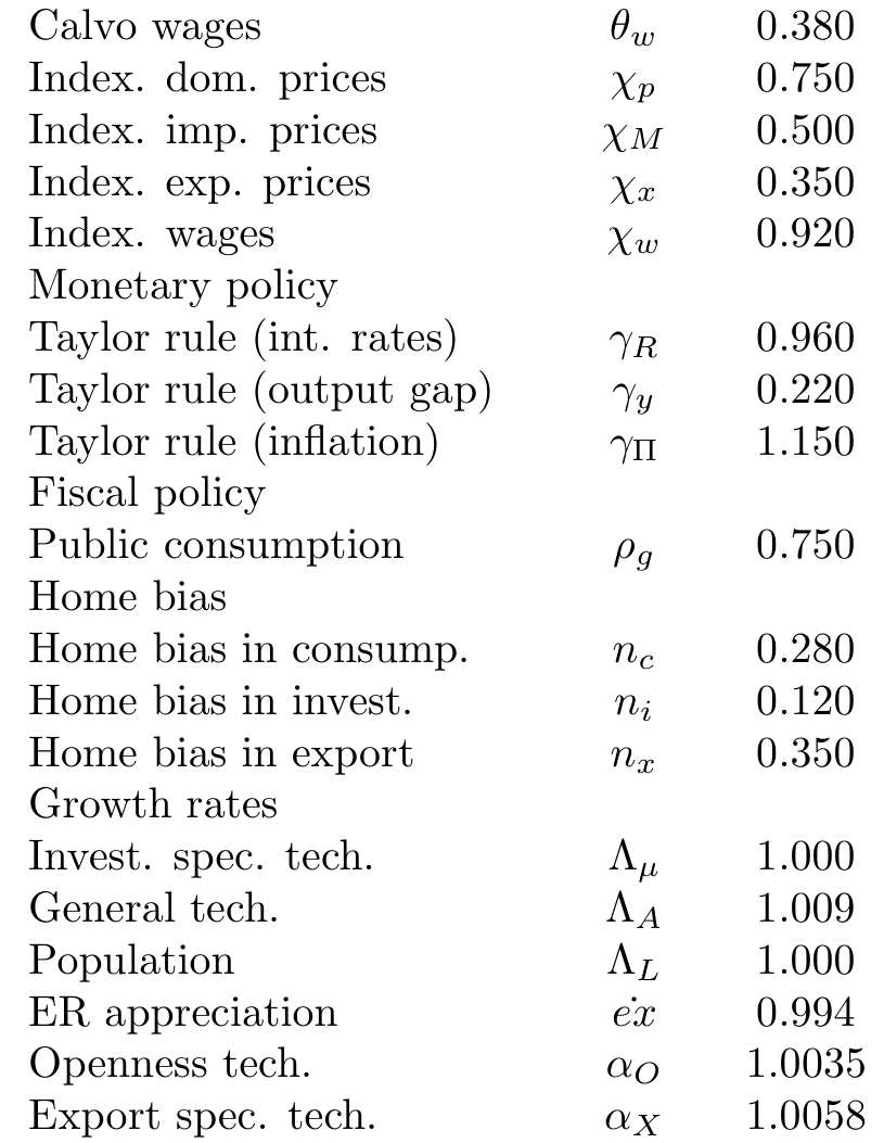
Calibration uncertainty: meta needed!

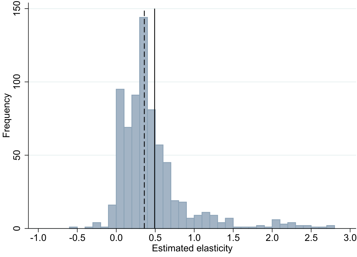
Estimates of the labor supply elasticity vary

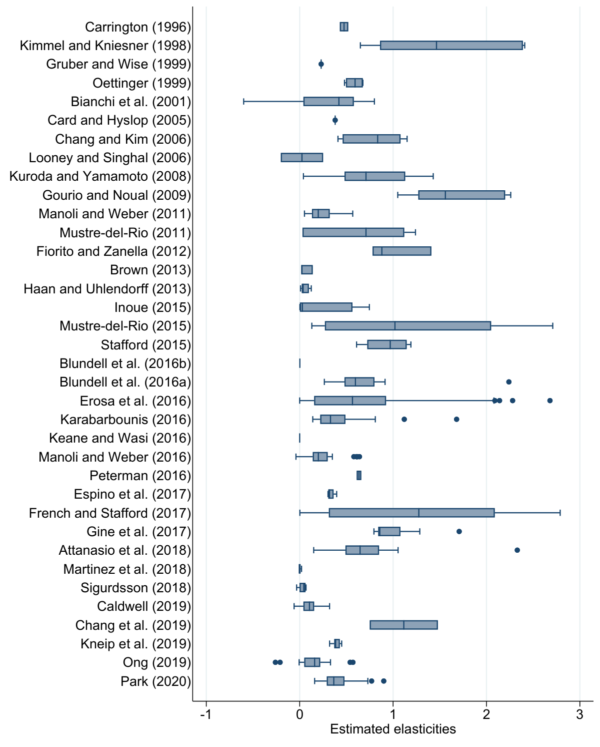
Values around 0.4 to 0.5 used for calibration (CBO)

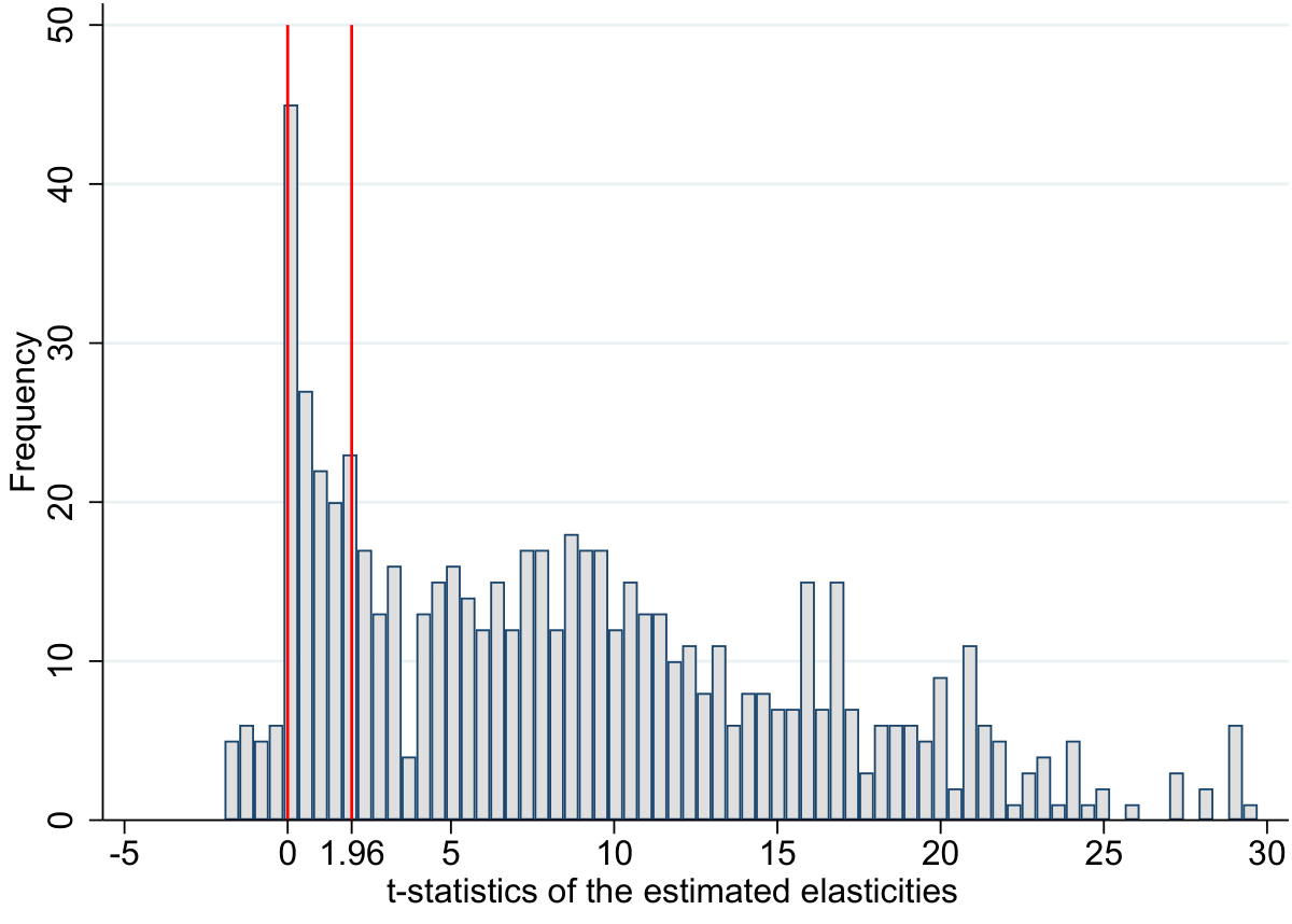
Bias: some estimates less likely to be reported

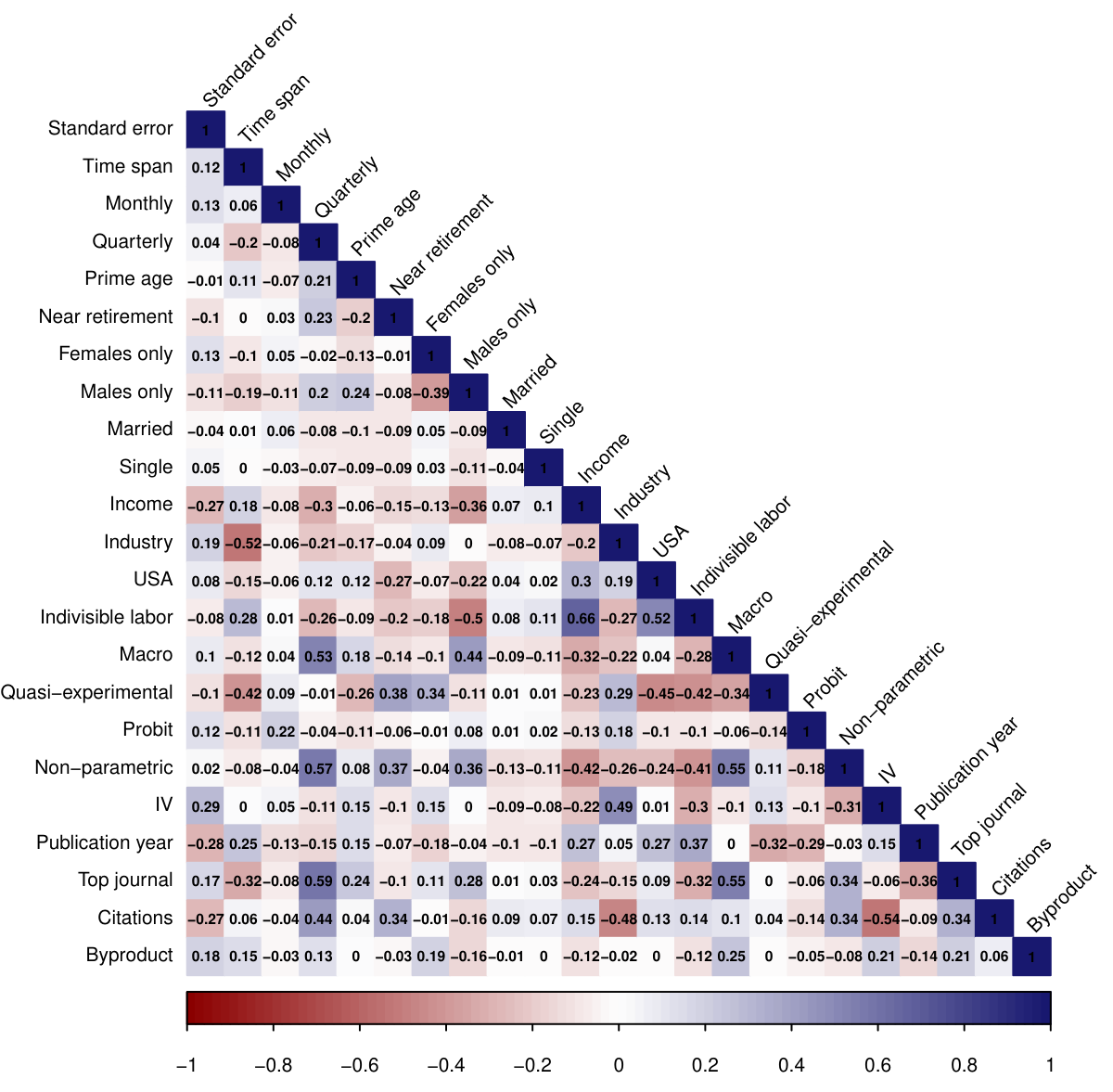
Context: different situations yield different estimates

Implied elasticity: taking bias and context into account

Let's construct a hypothetical study that uses all information reported in the literature but puts more weight on selected aspects (high precision, credible identification, etc.)

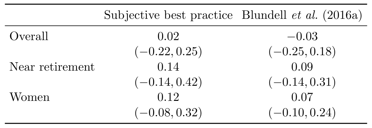
Guidelines

Guiding example: effect of beauty on success

Hands on

Open Stata and R

Results

1. Mean of 1,159 estimates from 67 studies: good looks → earnings ↑ 5%
2. Publication bias. After correction: 3%
3. Control for ability? Productivity? Beauty premium ≈ 1%

www.meta-analysis.cz/beauty

Revisions requested at Nature Human Behaviour.

Literature Search

Inspiration

Motivation example: increasing uncertainty

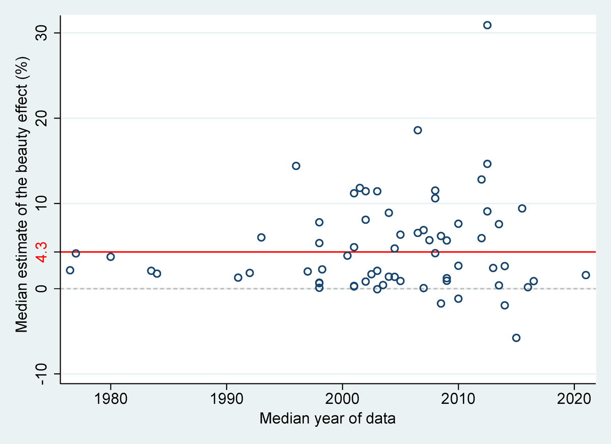
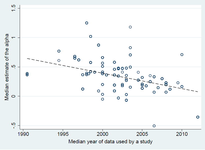
Motivation example: clear trend

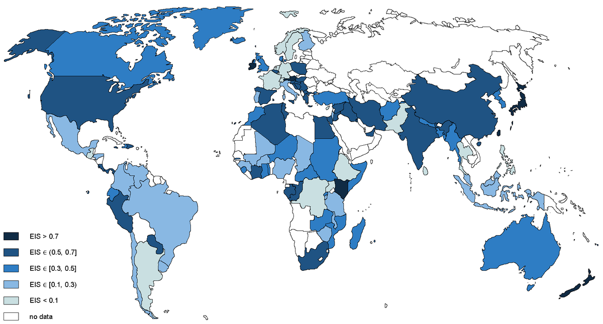
Motivation example: country-level differences

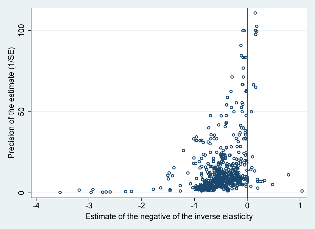
Motivation example: publication bias

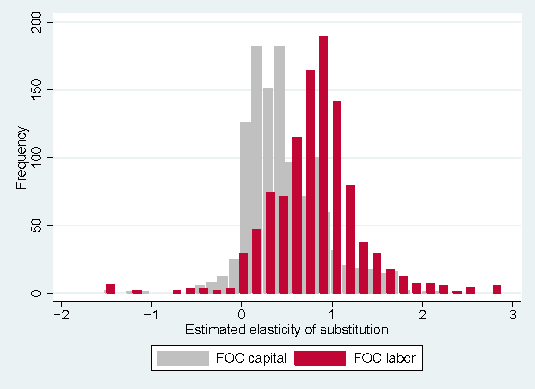
Motivation example: method heterogeneity

We use Google Scholar

Advantages:

• Full text, not just the abstract, title, keywords
• Inclusive
• Up-to-date

Disadvantages:

• Algorithm changes in time (replicability issues)
• Too many results
• Sometimes relevance unclear

Search steps (without AI for now)

1. Find 5 most relevant studies
2. Design a query that shows the 5 studies near the top
3. Go through first 500 hits
4. Read abstracts
5. Download potentially useful studies
6. Skim them
7. Repeat the procedure for the most recent studies (last 3 years)

Search query 1

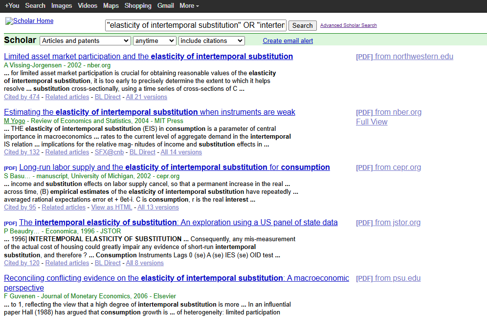
Search query 2

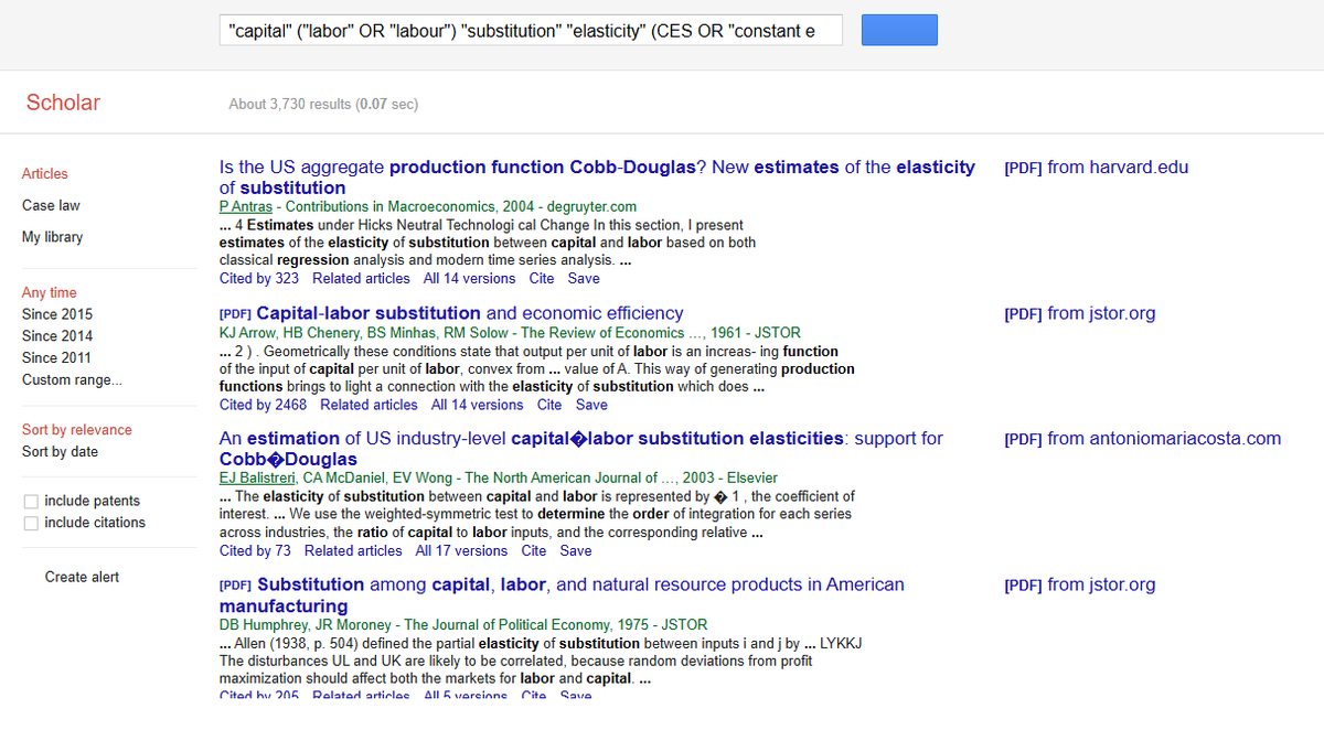
Primary studies

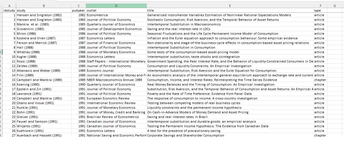
Snowballing

• No query is perfect
• Idea: cover studies not identified by the query but frequently mentioned in the literature
• For each primary study, download the list of references
• Inspect the 50 studies most frequently cited by the primary studies
• If you can use some of them, add them to your list

Snowballing example

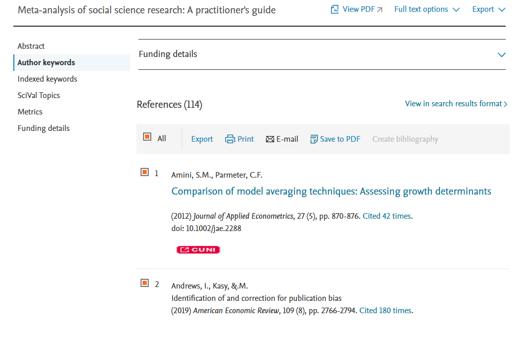
AI-enhanced literature search

1. Use Deep Research to explore recent literature and concepts
2. Ask ChatGPT thinking model to refine your Scholar query
3. Download 500 abstracts from Scholar or Publish or Perish
4. Let a ChatGPT Agent screen abstracts for relevant estimates
5. Ask Agent to download PDFs (or download manually)
6. Upload PDFs in batches of 5; ask which report usable estimates
7. (Optional) Use ASReview to double-check or co-train

Using thinking models to design Scholar query

• GPT thinking model helps refine search precision
• Prompt examples:
  • I want to do a meta-analysis of the beauty premium. Suggest a Google Scholar query to find empirical studies on attractiveness and income.
  • Too many irrelevant hits. How can I prioritize regression-based studies only?
• Output improves over iterations: clarify units, methods, outcomes, and keywords

Prompting ChatGPT Agent for screening

• Batch input: 20 to 50 abstracts at a time from Scholar export
• Example prompt: You are an expert in meta-analysis. For each abstract below and all other information you have about the paper, say whether the paper likely reports quantitative estimates on the effect of beauty on labor market outcomes that can be used in a meta-analysis. Justify briefly.
• Output: Paper 1: Yes (panel data, Table 2) Paper 2: No (conceptual) Paper 3: Maybe (ambiguous)

Screening PDFs for quantitative content

• Upload PDFs in small batches (e.g., 5 at a time)
• Example prompt: For each of these papers, does it contain new empirical estimates of the effect of beauty on wages that I can use in a meta-analysis? Point to specific tables or pages.
• Output format:
  • Paper A: Yes, Table 4, OLS and IV estimates on beauty premium
  • Paper B: No quantitative analysis
  • Paper C: Yes, appendix regression table

Optional enhancements and caveats

• Combine with ASReview for machine-assisted filtering
• Use Semantic Scholar for better metadata access
• Avoid over-reliance: AI helps, but expert judgment remains key
• Protect against false positives: Always validate flagged studies manually
• End-to-end AI infrastructure for meta-analysis: otto-SR
• AI duels for meta: https://github.com/tjhavranek/research-audit-duel-protocol
• Forthcoming MAER-Net guidelines on AI

Minimum requirements for meta-analysis

For modern meta-analysis techniques to work, you need at least:

1. 30 estimates
2. 10 studies
3. effect sizes
4. standard errors
5. sample sizes

What to do if I have, e.g., just 10 estimates from 4 studies? Focus on the median or weighted means.

Quality

• Some studies are published in poor journals or use weak identification. What to do?
• Option 1: exclude these studies ex ante. Not recommended.
• Option 2: include these studies with controls for journal quality and methodology. You can always exclude them as a robustness check.
• Note that some fields have standardized quality benchmarks (risk of bias)

Unpublished papers

• Try to collect all studies, published and unpublished
• If unfeasible, it is possible to focus just on published studies (fewer typos, peer-review)
• Including unpublished papers unlikely to alleviate publication bias
• Still too many papers? Recruit a co-author, AI, or use a random subset (last resort)

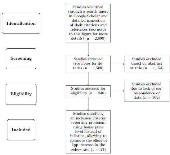
PRISMA: document your literature search

Data Collection

Effects must be quantitatively comparable

What does it mean?

• When we compare estimates reported in Study 1 and Study 2, it must be clear which one is larger
• It must be clear how much larger it is
• t-statistics are not useful measures of effect size
• Regression coefficients are not comparable in general if studies use different units

Elasticities

x-elasticity of y: ε = ((∂ y)/y)/((∂ x)/x)

P-elasticity of Q: ε = ((∂ Q)/Q)/((∂ P)/P) if continuous

ε = ((Q_2 - Q_1)/Q_1)/((P_2 - P_1)/P_1) = (% change in quantity Q)/(% change in price P) if discrete

Elasticities can be recovered from regressing log(Y) on log(X).

Semi-elasticities, dollar values, std.dev. changes

• Semi-elasticity: effect of euro adoption on trade, effects of foreign investment on domestic productivity, effects of borders on trade
• Dollar values: statistical value of life, social cost of carbon
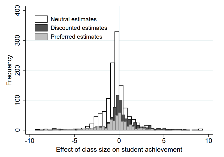
• Std.dev. changes: effect of class size on student test scores. What to do here?
• Class size is measured the same way in all studies (number of kids).
• Test scores are measured differently.
• Solution: By how many standard deviations do test scores improve if we decrease class size by 10 students?

Standardized mean differences

θ = (μ_1 - μ_2)/σ, where μ_1 is the mean for one population, μ_2 is the mean for the other population, and σ is a standard deviation based on either or both populations.

• Very popular in psychology, not much used in economics. Why?
• For many questions the treatment and control are not binary classifications (we look at the intensity of treatment)

Partial correlation coefficients

Example: tuition fees and university enrollment. Ideally, we would need price elasticities of demand (PED), but many studies are not log on log.

So we transform the estimates to partial correlations using t-statistics and degrees of freedom:

PCC(PED)_ij = (T(PED)_ij)/(√(T(PED)_ij^2 + DF(PED)_ij)).

PCC caveats

• Last resort: can be used almost always, but we lose a lot of information
• Difficult to interpret (some guidelines provided by Doucouliagos, 2011)
• Statistical problems for meta-analysis methods (but this is the case also for SMD)
• Include robustness checks: e.g. a subsample of elasticities in the case of tuition fees and university enrollment

Collect all estimates

Standard errors

• Absolutely crucial for meta-analysis
• If not reported directly, can be computed from t-statistics or p-values
• Last resort: approximation based on within-study variation (Matousek et al. 2022)
• Interactions, transformations: delta method

AI-assisted data collection: Overview

• As of March 2026, human review still essential
• AI reasonably good at
  • Identifying key study dimensions (estimation method, outcome type, etc.)
  • Extracting basic data with structured prompts and examples
  • Reducing workload to a single reviewer
• Tools: ChatGPT thinking, Agent Mode, NotebookLM
• End-to-end AI infrastructure for meta-analysis: otto-SR
• Don't rely on one model (add Claude, Gemini, Grok)!!

Step-by-step data collection workflow

1. Use Deep Research + thinking model to find key coding dimensions
2. Examples: OLS vs IV, cross-section vs panel, outcome types, country, controls
3. Upload a few example PDFs + your coded spreadsheet to ChatGPT Agent
4. Prompt Agent: "Extract these columns from new PDFs using my examples as a guide."
5. Refine extraction prompts based on feedback
6. Use NotebookLM as an independent extraction check
7. Validate discrepancies manually; spot-check the rest

Example prompt for PDF data extraction

Here are 3 PDFs and the corresponding rows from my meta-analysis data sheet. Learn the structure. These data are collected well and I want you to collect data from other papers. I will send 5 new PDFs. Extract estimates of the beauty premium and the corresponding standard error. Collect information on the estimation method used, the definition of the beauty variable, definition of the earnings variable.

• Agent mode allows memory and consistency across batches
• Output can be verified, adjusted, and exported as CSV
• See summary on MAER-Net website.

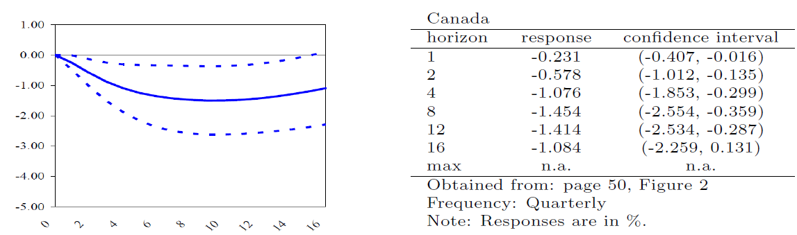
Graphical estimates, measurement error

Details: Ehrenbergerova et al. (2023, IMF Economic Review)

Outliers

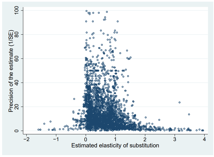
What to do with outliers?

• No consensus
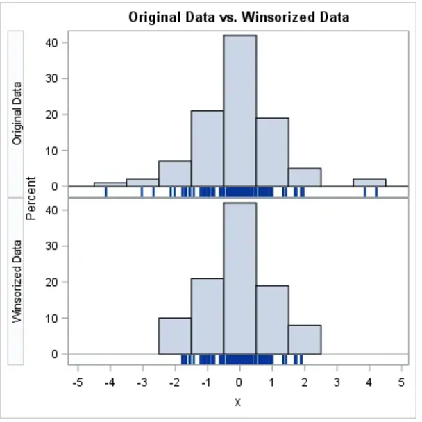
• Approach 1: omit very large effects (and standard errors), e.g. more than 3 standard deviations away from the mean
• Approach 2: run robust meta-regression or use tools for outlier detection in regression
• Approach 3: use winsorizing (my personal preference)
• Always report robustness checks

Winsorization

Hands on

Open Stata

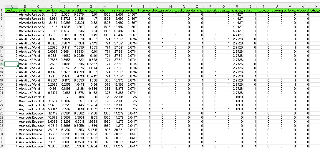
Reflecting context: the effect of beauty on success

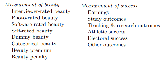
Measurement

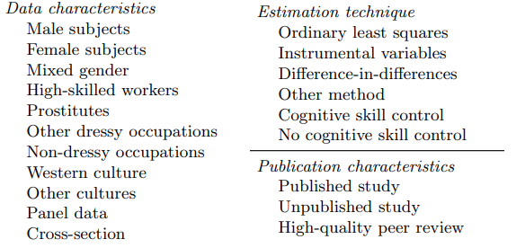
Data, estimation, publication

Value added

• Meta-analysis can be used to test hypotheses that primary studies cannot investigate
• Example: the effect of daylight saving time on energy consumption
• Individual studies have data for individual countries (or provinces)
• In meta-analysis, we have data for dozens of countries
• We can investigate the sources of cross-country differences

DST savings and latitude

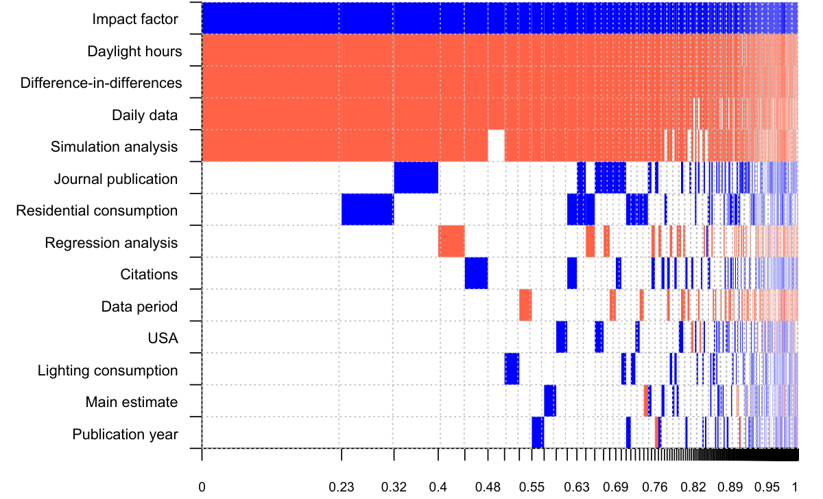
Conventional Tools

Summary statistics for meta-analysis

• Simple mean of reported estimates: natural starting point
• But inefficient and affected by outliers, publication bias, p-hacking
• Median: surprisingly robust to most problems in meta-analysis
• If you have only a few studies or estimates, focus on the (unweighted) median!
• Classical meta-analysis approach: use inverse variance as the weight

More precision -> more weight

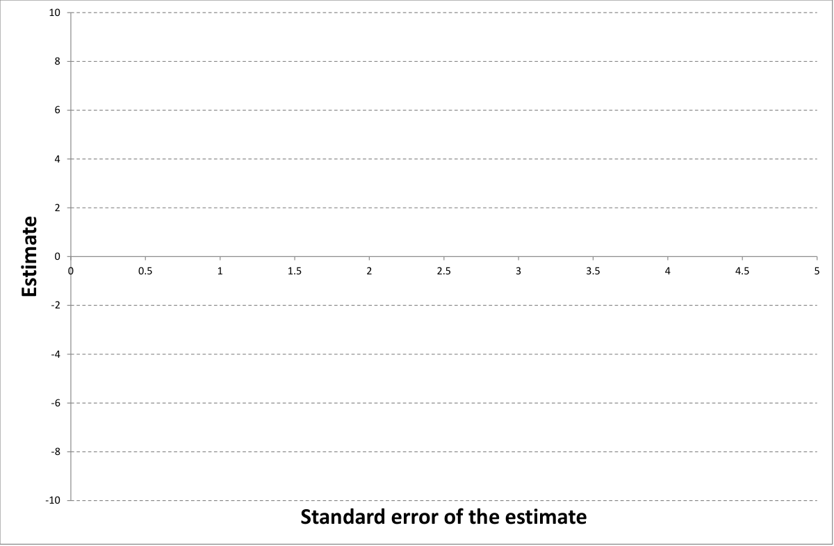
More precision -> more weight

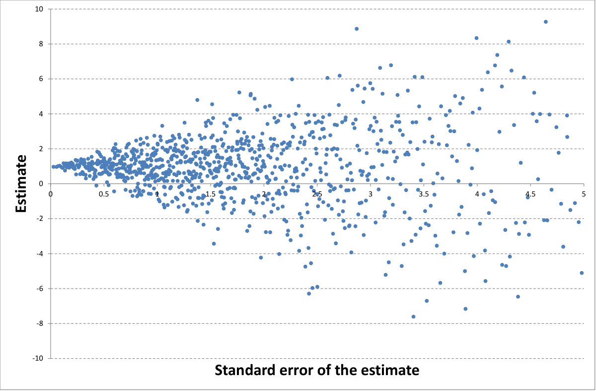
More precision -> more weight

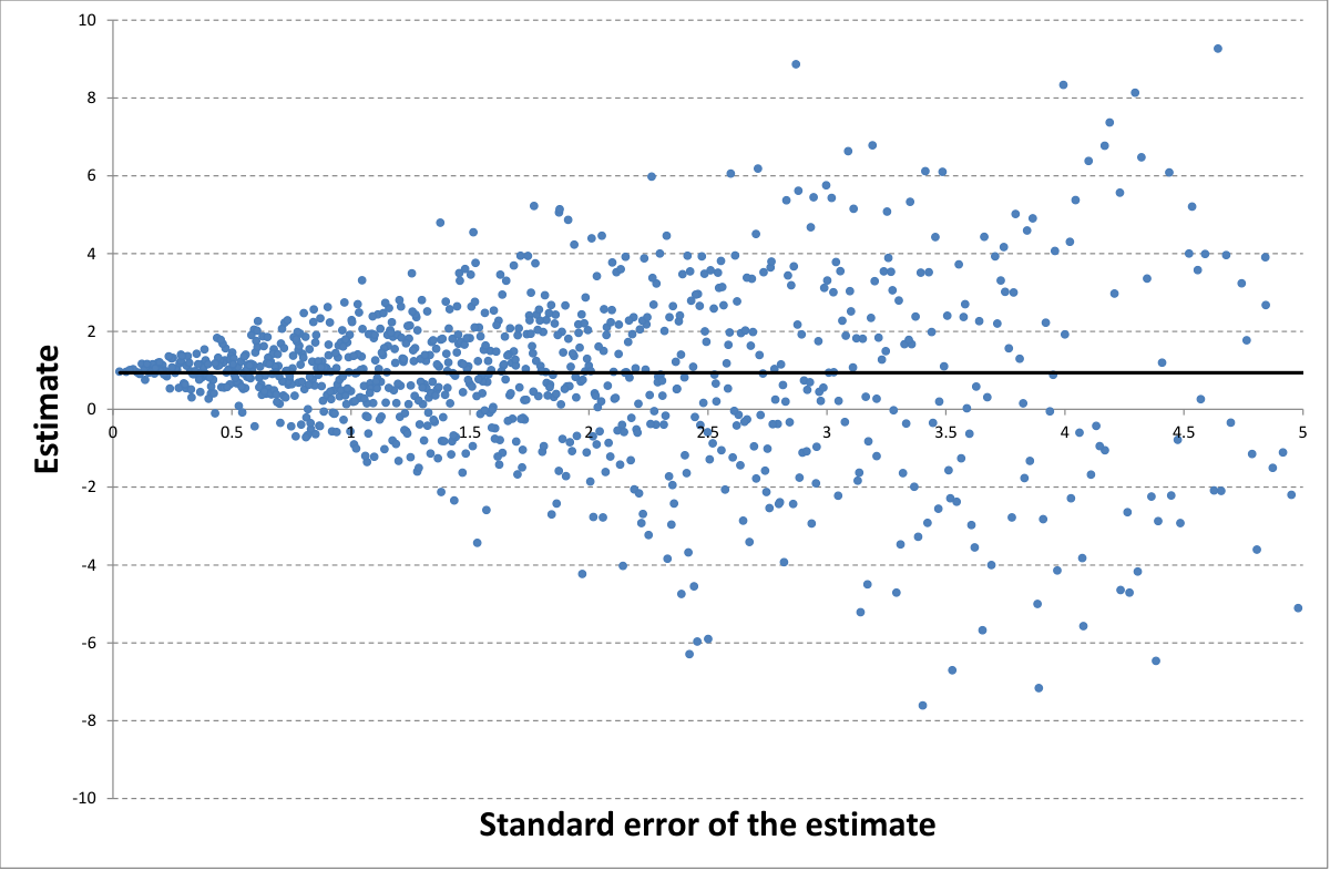
“Fixed effect” estimator in meta-analysis

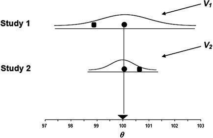
“Fixed effect” estimator in meta-analysis

Mean weighted by inverse variance of individual estimates. Very sensitive to outliers in precision (including typos). Y_i = θ + ε_i, (1); V_i = σ^2/n, (2); W_i = 1/V_i, (3); M = (Σ_(i=1)^k W_i Y_i)/(Σ_(i=1)^k W_i), (4); V_M = 1/(Σ_(i=1)^k W_i). (5)

Hands on

Open Stata

FE vs. UWLS: point estimate

• Unrestricted weighted least squares yield the same point estimate: θ̂ = (Σ w_i θ_i)/(Σ w_i), w_i = 1/SE_i^2
• Difference: Variance estimation.

Method | Point Estimate
Fixed-Effect (FE) | θ̂ = (Σ w_i θ_i)/(Σ w_i)
UWLS | θ̂ = (Σ w_i θ_i)/(Σ w_i)

Same estimate, different variance!

FE vs. UWLS: variance

Feature | Fixed-Effect (FE) | UWLS
Assumption | Identical θ | Allows heterogeneity
Variance formula | 1/(Σ w_i) | (Σ w_i (θ_i - θ̂)^2)/(Σ w_i)
Variance components | Within-study only | Within + between-study
Robustness | Sensitive to misspecification | More robust

FE typically underestimates variance. Use UWLS!

Correction. The UWLS variance of the pooled estimate is Σ w_i (θ_i - θ̂)^2 / ((k - 1) Σ w_i); the table leaves out the factor k - 1. This is the formula for independent estimates: with several estimates per study, use standard errors clustered by study, as the course code does.

Fixed effect

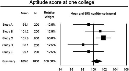
Random effects

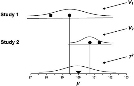
Random effects

The weight is now diluted by a heterogeneity term. More robust to outliers in precision and heterogeneity, less robust to publication bias. Y_i = μ + ξ_i + ε_i, (1); V_i = σ^2/n, (2); W_i = 1/(V_i + τ^2), (3); M = (Σ_(i=1)^k W_i Y_i)/(Σ_(i=1)^k W_i), (4); V_M = 1/(Σ_(i=1)^k W_i). (5)

Estimating τ^2 in random-effects model

Between-study variance τ^2 accounts for heterogeneity across studies. Common estimators:

• DerSimonian-Laird (DL): τ^2_DL = (Q - (k - 1))/C, C = Σ w_i - (Σ w_i^2)/(Σ w_i). Simple, but underestimates τ^2 when k is small.
• Restricted Maximum Likelihood (REML): max_τ^2 Σ log (w_i^* + τ^2) + Σ ((y_i - θ̂)^2)/(w_i^* + τ^2). More accurate, default in software.

Rule of thumb: Use REML unless simplicity is needed!

Correction. The REML line is not the restricted likelihood. REML chooses τ^2 ≥ 0 to minimise Σ log(v_i + τ^2) + log Σ W_i + Σ W_i (y_i - θ̂)^2, where v_i are the within-study variances, W_i = 1/(v_i + τ^2) and θ̂ is the weighted mean; software solves this numerically. A negative DL estimate is set to zero.

Random effects

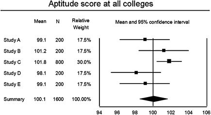
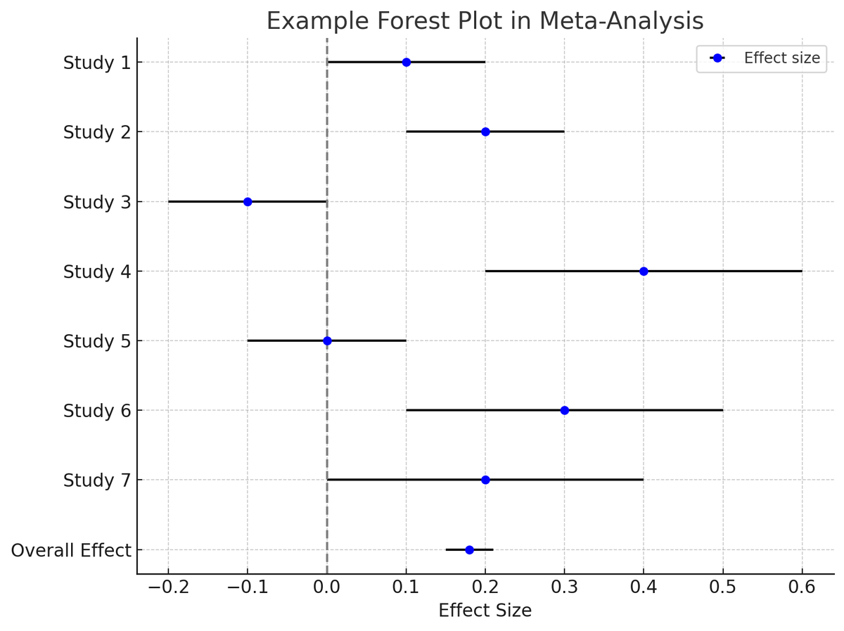
Forest plot

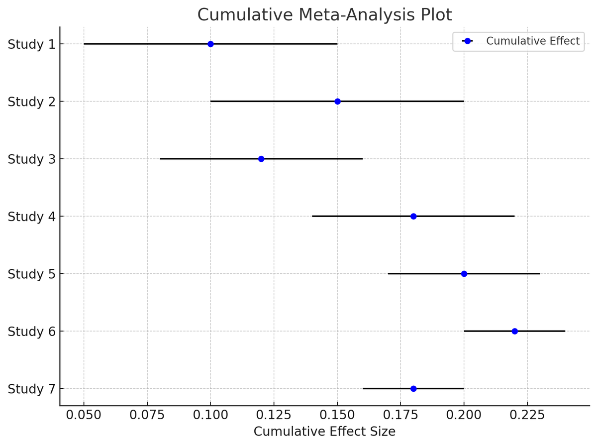
Cumulative meta-analysis plot

Publication Bias

Paxil scandal

• Background:
  • Paxil (paroxetine): Antidepressant approved for adolescents, developed by GlaxoSmithKline (GSK).
  • Study 329 (1998-2001): Clinical trial funded by GSK to test Paxil's safety and efficacy in adolescents.
• What Happened?
  • Published study claimed Paxil was "well-tolerated and effective."
  • Internal documents later revealed:
    • Negative results (e.g., increased suicidal ideation) were downplayed.
    • Positive outcomes were selectively reported.

Correction. The FDA never approved paroxetine for patients under 18: it was approved for adults and promoted for adolescent depression. Study 329 ran from 1994 to 1998 and was published in 2001; the independent reanalysis appeared in 2015.

Paxil scandal

• Discovery of Bias:
  • Legal proceedings in 2012 forced disclosure of internal data.
  • Independent reanalysis of Study 329 showed:
    • No significant benefit over placebo.
    • Serious safety concerns (e.g., suicidal ideation).
• Key Lessons:
  • Publication bias can harm patients and public trust.
  • Highlights the need for:
    • Transparency in research data.
    • Independent replication and reanalysis.

No bias, no E-SE correlation (?)

Researchers estimate

Earnings_j = γ Beauty_j + … + w_j.

They assume that γ̂/SE_γ̂ has a t-distribution.

→ estimates should not be correlated with standard errors (Card & Krueger, 1995)

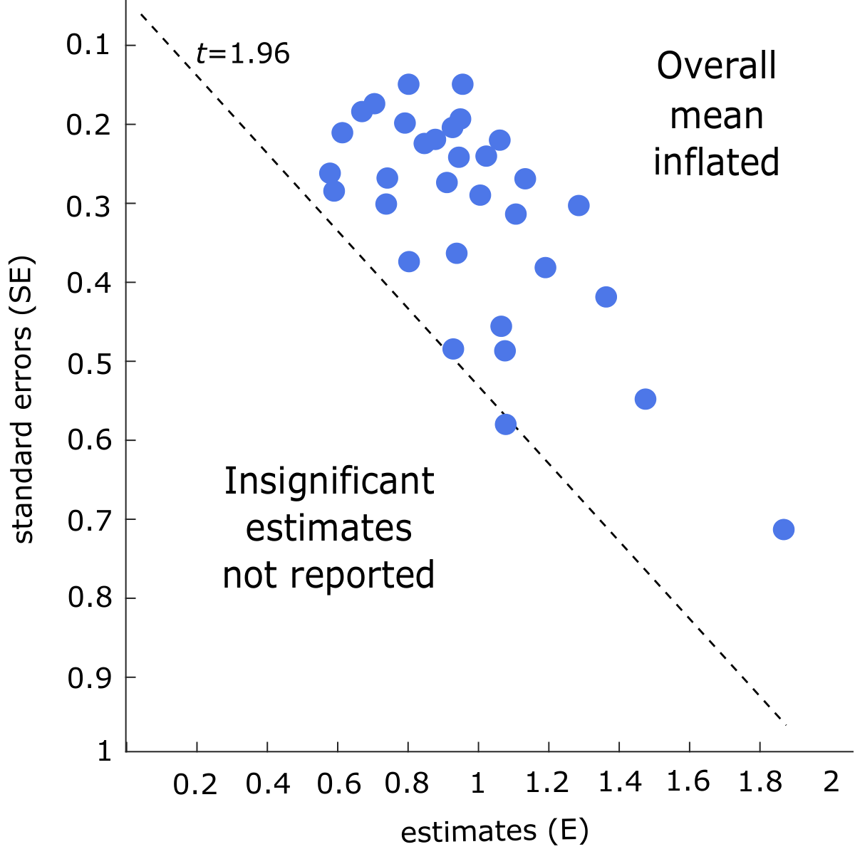
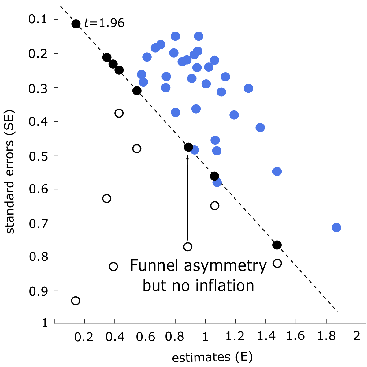
Type I: Selection for the “correct sign.” Type II: Selection for statistical significance.

Simulation

Simulation

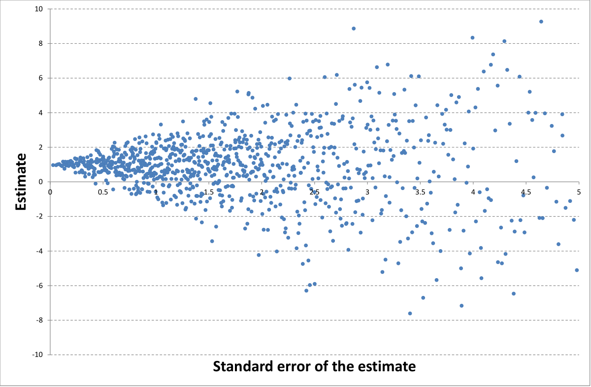
Simulation

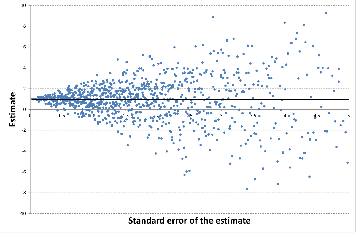
Simulation

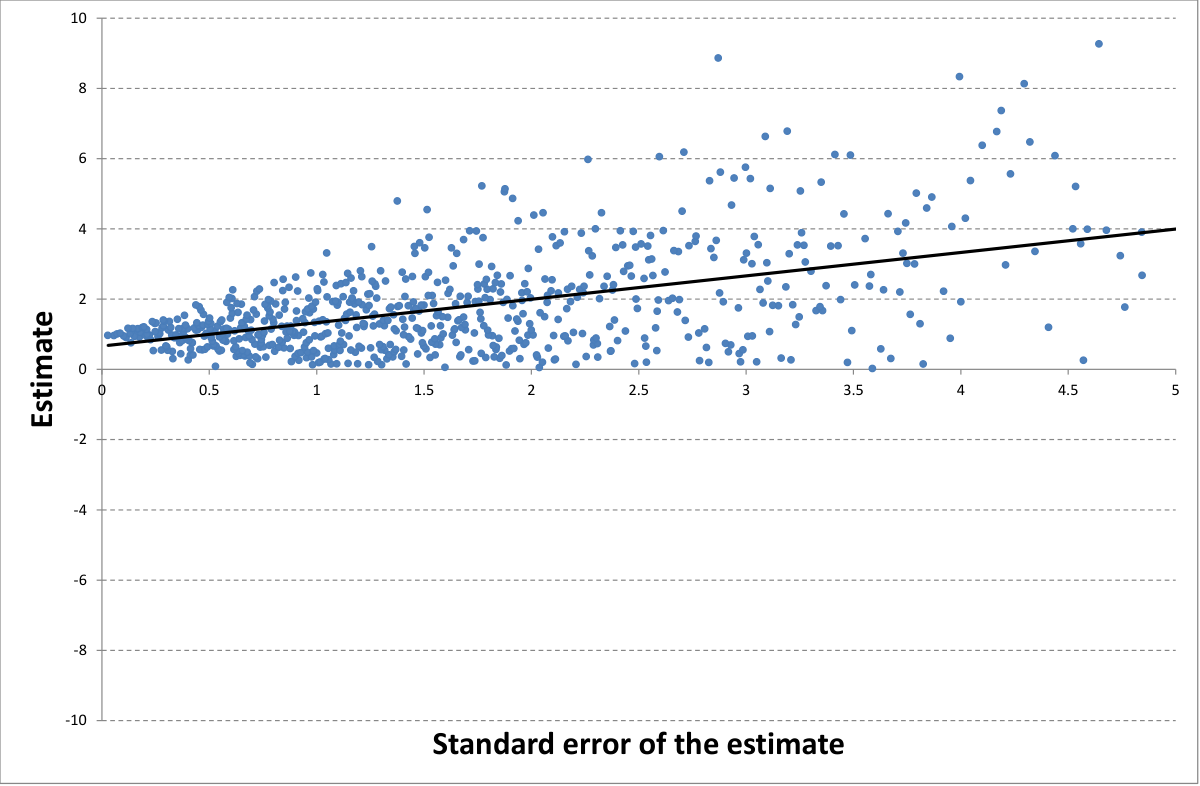
Simulation

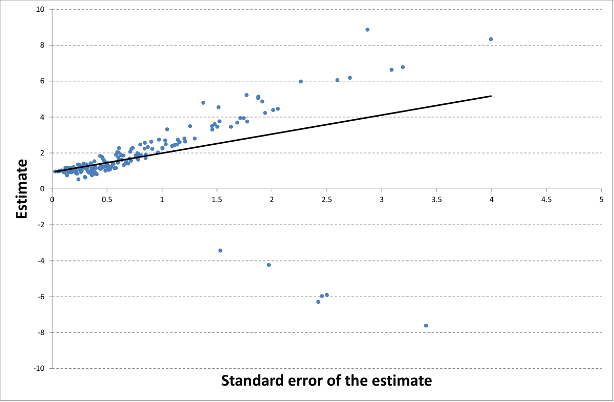
Simulation

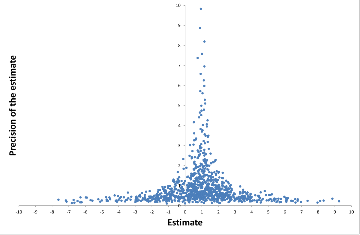
Simulation

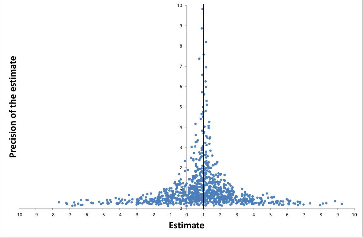
Simulation

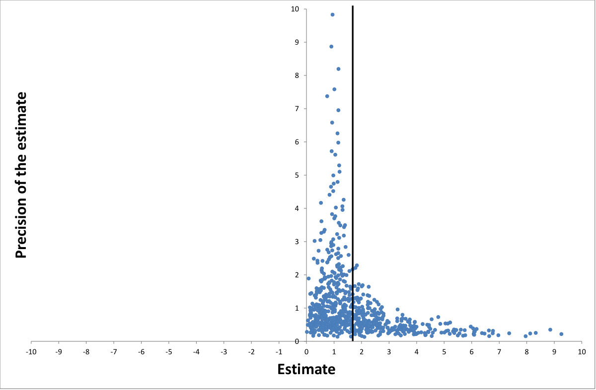
Simulation

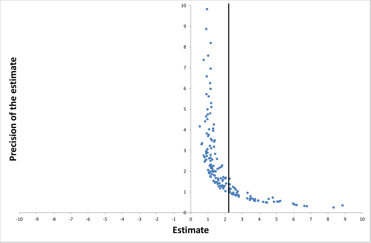
Funnel asymmetry test

In the absence of publication bias the funnel should be symmetrical: estimate_i = β [true effect] + β_0 SE_i [publication bias] + μ_i.

The equation is heteroscedastic. Weighted least squares yield

t_i = β_0 + β (1/SE_i) + ϑ_i. This is called the funnel asymmetry test, precision effect test (FAT-PET).

Hands on

Open Stata

Default nonlinear correction model (PEESE)

Publication bias unlikely to be linear in SE. Precision effect test with standard error:

estimate_i = β [true effect] + β_0 SE^2_i [publication bias] + μ_i.

Weighted least squares yield

t_i = β_0 SE_i + β (1/SE_i) + ϑ_i.

Works well under most circumstances.

WAAP (Ioannidis et al., 2017)

Weighted Average of Adequately Powered (WAAP) estimates.

• Focus on studies with adequate statistical power to reduce the impact of selective reporting.
• Combines results only from studies with at least 80% power.

Issues:

• Simple and robust.
• Need to estimate the true effect first and then compute power.

Stem-based correction technique (Furukawa, 2019)

Stem-based method:

• A non-parametric estimator that exploits the variance-bias trade-off.
• Focuses on the most precise estimates, referred to as the “stem” of the funnel plot.

Key features:

• Robust to various publication selection processes.
• Does not rely on specific distributional assumptions.

Application:

• Filters studies with the highest precision (lowest standard errors) to estimate the true effect.
• Reduces influence from noisier, potentially biased studies in the broader funnel plot.

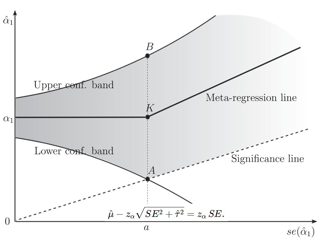
Endogenous kink model (Bom & Rachinger, 2019)

Overview:

• Fits a piecewise linear model with a kink determined by the data.
• Identifies where publication selection is less likely to occur.

Key features:

• Endogenously estimates the cutoff based on standard errors.
• Often reduces bias and improves efficiency compared to traditional methods.

Application:

• Highlights genuine effects by focusing on less selective segments of the data.
• Effective in meta-analyses with substantial heterogeneity in study precision.

Endogenous kink

Selection model (Andrews & Kasy, 2019)

Overview:

• Models the selection process explicitly to address publication bias.
• Assumes researchers are more likely to publish statistically significant results.

Key features:

• Uses the likelihood of publication as a function of statistical significance.
• Adjusts estimates to reflect the missing studies.

Comparison to funnel-based models:

• Selection models are more rigorous but require stronger assumptions about the publication process.
• Funnel methods are simpler and more robust to model misspecification.

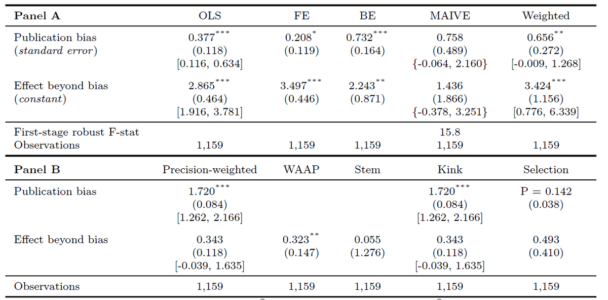
Beauty effect: corrected mean probably below 3

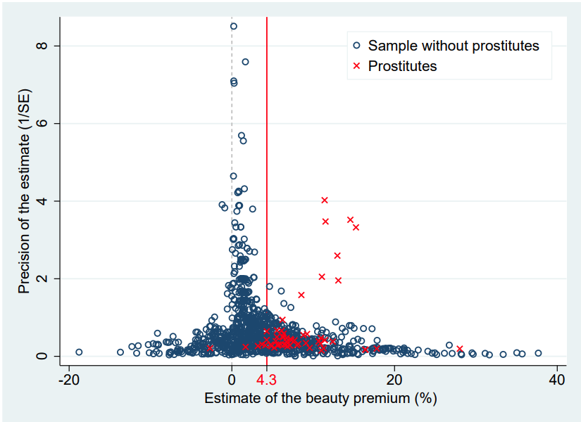
Sex workers stand apart

Bias caused by selection for a positive sign

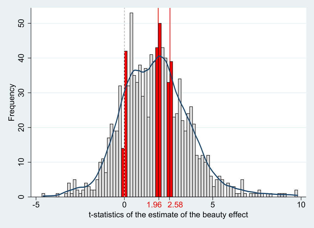
P-hacking

Web app for p-hacking correction: EasyMeta.org

Recall publication bias

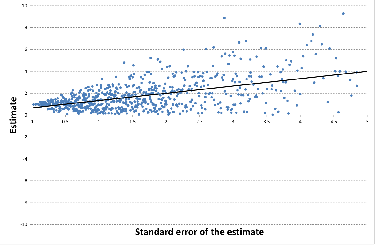
Recall publication bias

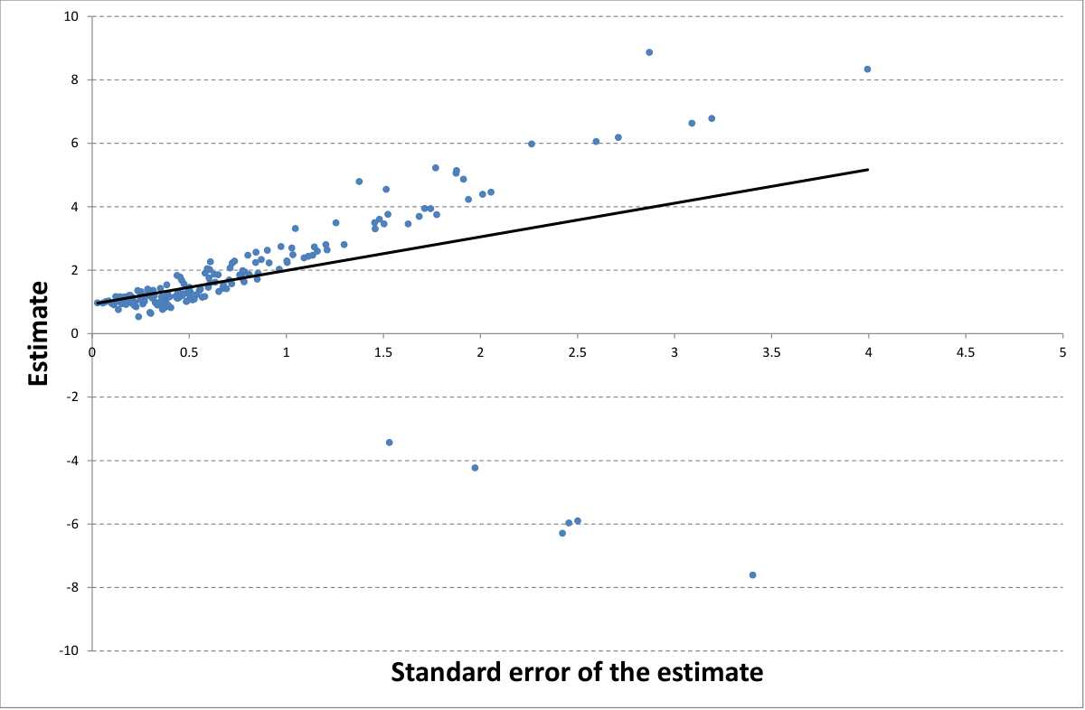
Key difference

• Publication bias: all estimates are individually unbiased
• The entire literature is biased because estimates are selectively reported
• If we know publication probabilities, we can recover the true effect (selection models)
• P-hacking: individual estimates can be biased
• Classical selection models fail
• Funnel-based models can work (with adjustments)

Example: education premium

True model: Earnings_j = γ Education_j + δ Ability_j + v_j,

Omitted variable: Earnings_j = γ Education_j + w_j,

Proxy: Earnings_j = γ Education_j + ω IQ_j + x_j,

Instrument: Earnings_j = γ Education_j + z_j, Distance_j

Ability not observed.

Primary studies:

1. ignore ability → γ̂ too large, SE(γ̂) too small.
2. include a proxy → γ̂ smaller, SE(γ̂) larger.
3. quasi-experiment → γ̂ even smaller, SE(γ̂) even larger.

(With a diagram, in the PDF.)

Some estimates spuriously large & precise

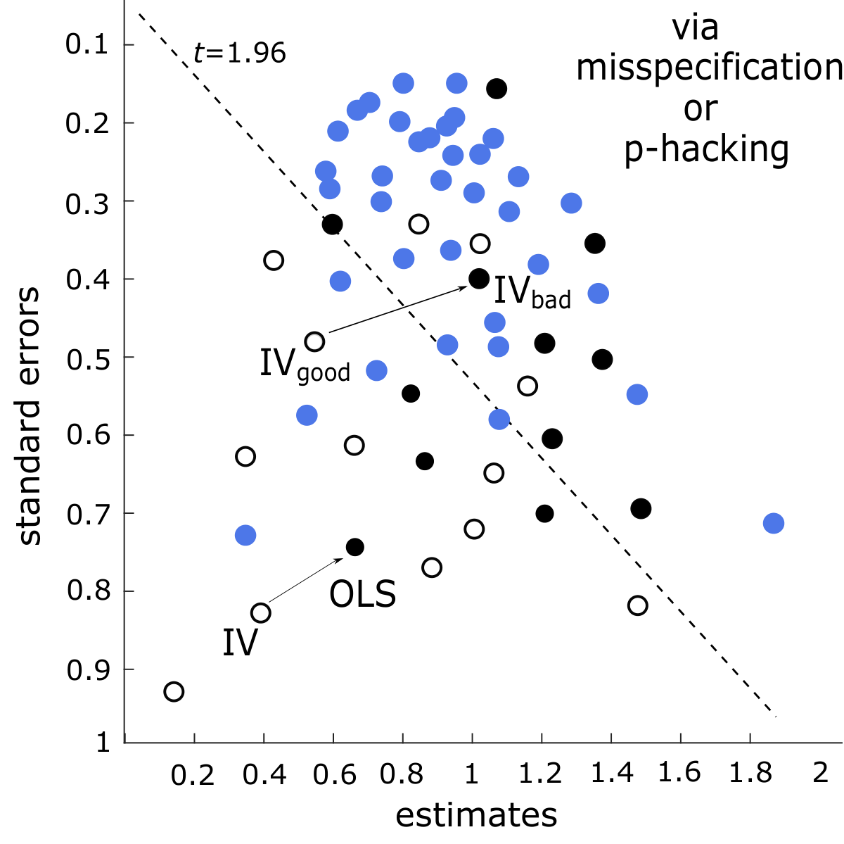
All estimators biased upwards

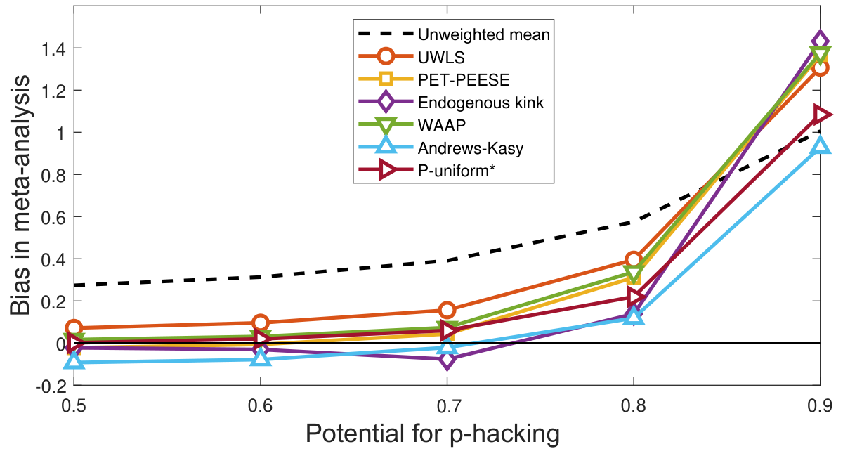
Example: Changing controls changes precision

Regression of test scores on class size

 | (1) | (2) | (3) | (4)
Small class (treatment) | 4.82 | 5.37 | 5.36 | 5.37
 | (2.19) | (1.26) | (1.21) | (1.19)
White/Asian |  |  | 8.35 | 8.44
 |  |  | (1.35) | (1.36)
Girl |  |  | 4.48 | 4.39
 |  |  | (0.63) | (0.63)
Free lunch |  |  | -13.15 | -13.07
 |  |  | (0.77) | (0.77)
White teacher |  |  |  | -0.57
 |  |  |  | (2.1)
Teacher experience |  |  |  | 0.26
 |  |  |  | (0.10)
Master's degree |  |  |  | -0.51
 |  |  |  | (1.06)
School intercepts | No | Yes | Yes | Yes
Sample | 5,861 | 5,861 | 5,861 | 5,861

Notes: Adapted from Krueger (1999). Dependent variable: test score percentile. Standard errors in parentheses.

Changing clustering changes precision

Regression of test scores on class size

 | Krueger (1999) | Replications using different computations of SE
 | (1) | (2) | (3) | (4) | (5) | (6)
 |  | Bootstrap of | Class | School | Huber-White | Plain vanilla
 |  | class clusters | clusters | clusters | SE | SE
Small class | 4.82 | 4.71 | 4.71 | 4.71 | 4.71 | 4.71
 | (2.19) | (2.00) | (1.88) | (1.38) | (0.79) | (0.76)
Sample | 5,861 | 5,743 | 5,743 | 5,743 | 5,743 | 5,743

Notes: Dependent variable: test score percentile. Standard errors (SE) in parentheses.

Available at meta-analysis.cz/class. (forthcoming in JOLE)

Funnel plot

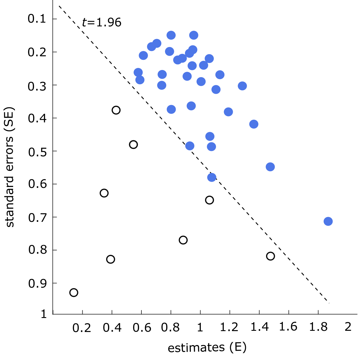
Publication bias

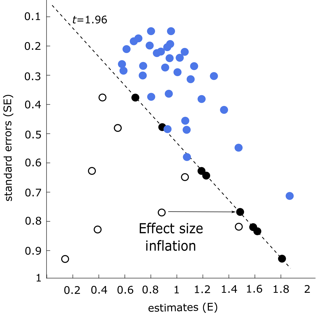
Conventional p-hacking

Spurious precision

Key meta assumption broken

PEESE:

Ê_i = E_0 + β SE(Ê)^2_i + u_i,

corr(SE,u) ≠ 0 ⇒ β̂ and Ê_0 biased.

Natural solution: N instrumenting SE(Ê)_i^2 → MAIVE.

(With a diagram, in the PDF.)

Options for the meta-analyst

1. Use only quasi-experimental studies.
2. Include controls (dummies for OLS, DID, …). But in observational research we never know the true model!
3. Remove “bad” variation from SE → MAIVE.

Meta-analysis instrumental variable estimator

MAIVE intuition: Ê_i = E_0 + β SE(Ê)^2_i + u_i, where the standard error, by definition, depends on 1/N_i.

MAIVE first stage: SE(Ê)^2_i = α_0 + α_1 (1/N_i) + π_i, where π_i stands for hacking or misspecifications.

MAIVE adjustment: SE(Ê)^2_(adj,i) = α̂_0 + α̂_1 (1/N_i). On the slide, π_i and its label, hacking or misspecifications, are struck out: the adjusted standard error keeps only the part explained by sample size.

• MAIVE + PEESE = classical IV.
• Can add controls in the 2nd stage.
• Plug MAIVE-adjusted SEs into other estimators.

(With a diagram, in the PDF.)

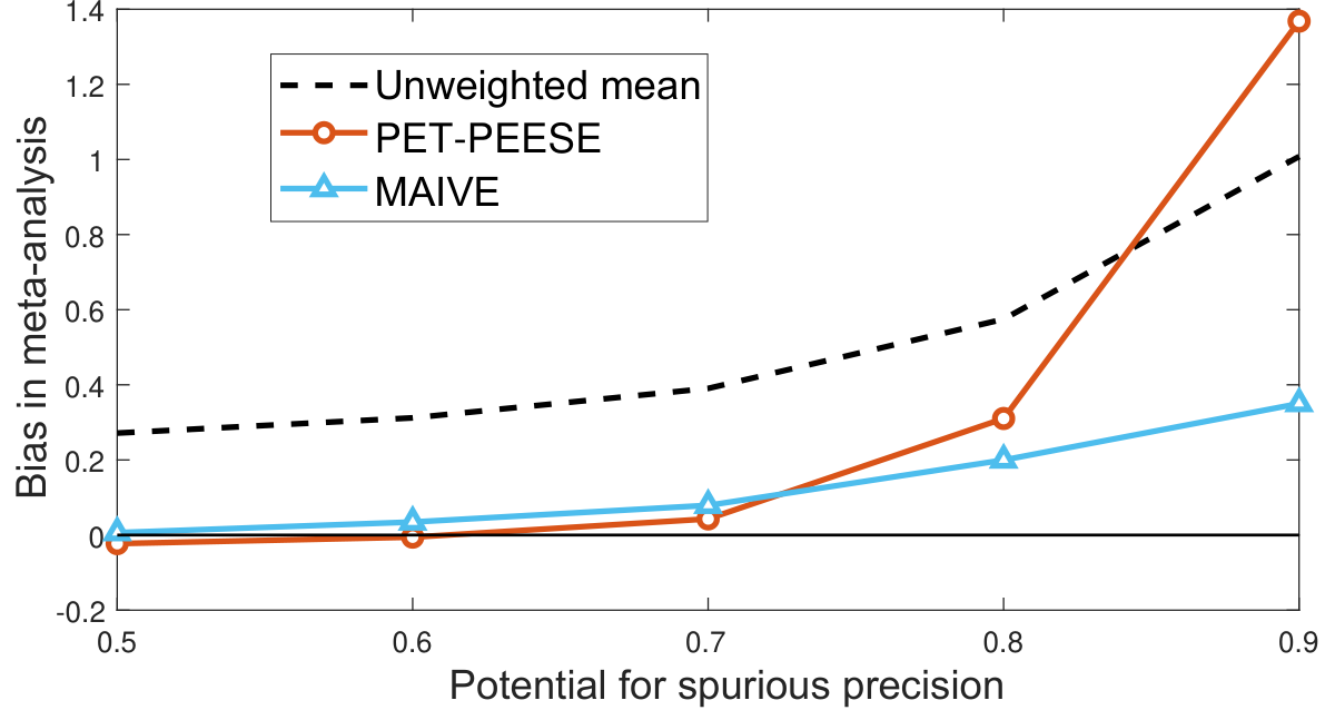
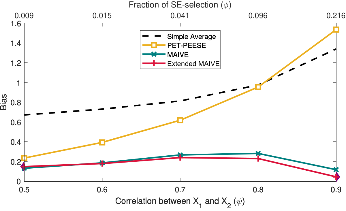
MAIVE alleviates the bias

Extended MAIVE (WAIVE: Weighted Adjustment)

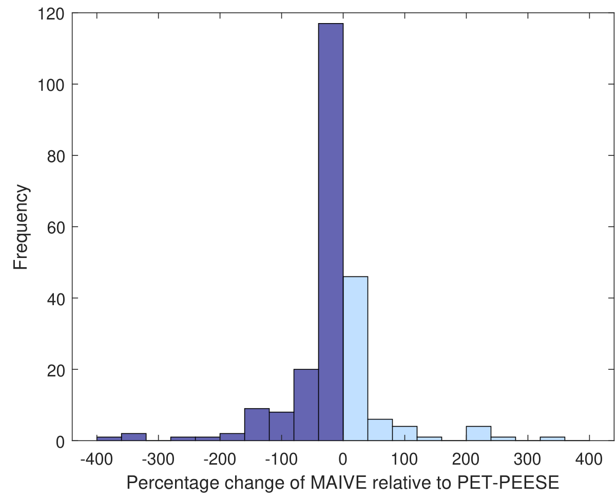
MAIVE reduces PET-PEESE in 70% of the cases

Practical issues

• Can methods or p-hacking influence both Ê and SE?
• Yes → MAIVE helps.
• No → MAIVE doesn't hurt much.

meta-analysis.cz/maive

Published in Nature Communications.

Hands on

Open Stata (MAIVE web app at easymeta.org)

RTMA: Maya Mathur's p-hacking correction

• Right-truncated meta-analysis (Mathur 2024, RSM)
• Assumption 1: insignificant estimates are NOT p-hacked
• Assumption 2: estimates are normally distributed
• Assumption 3: there are enough insignificant estimates published that we can recover the underlying distribution
• Bayesian techniques used for computation feasibility (ML would typically need huge samples)
• Digression: Robust Bayesian Meta-Analysis (RoBMA)

Hands on

Open R

Heterogeneity

Guiding example: beauty and success

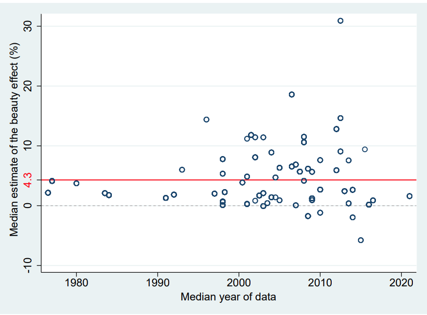
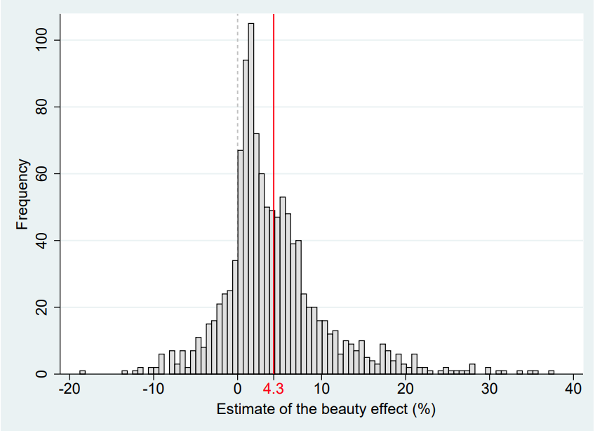
Heterogeneity both within and across

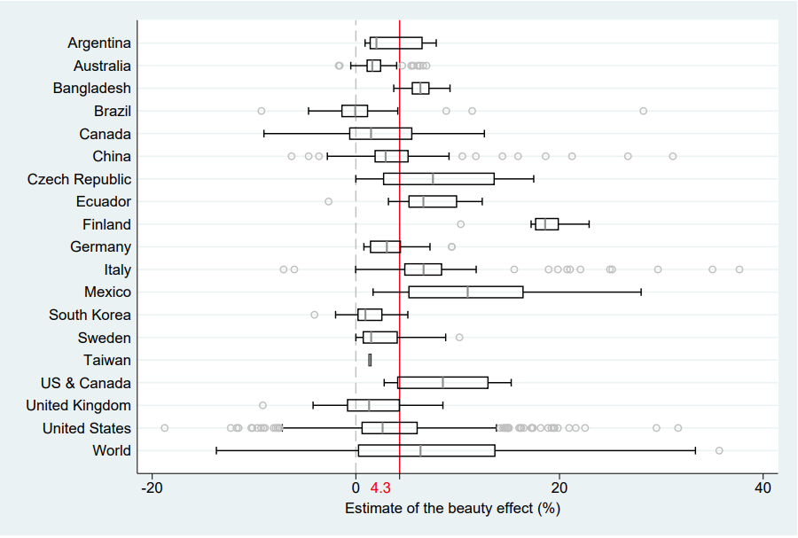
Wide dispersion

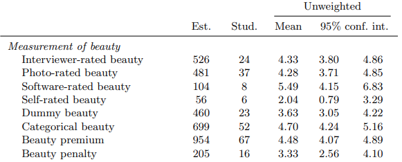
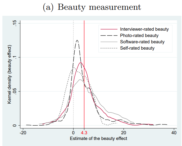
Measurement of beauty

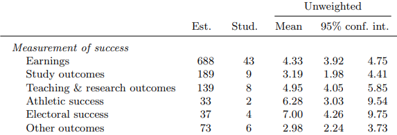
Measurement of success

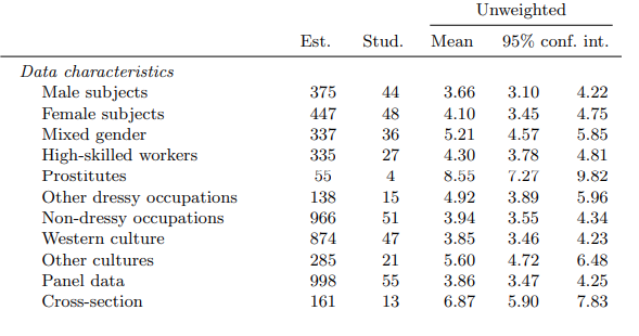
Data characteristics

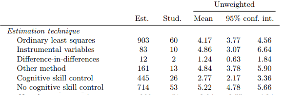
Estimation technique

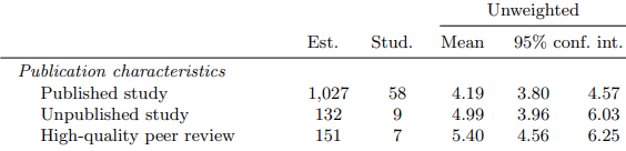
Publication characteristics

Beauty measurement doesn't matter

Hands on

Open Stata

Success measurement doesn't matter

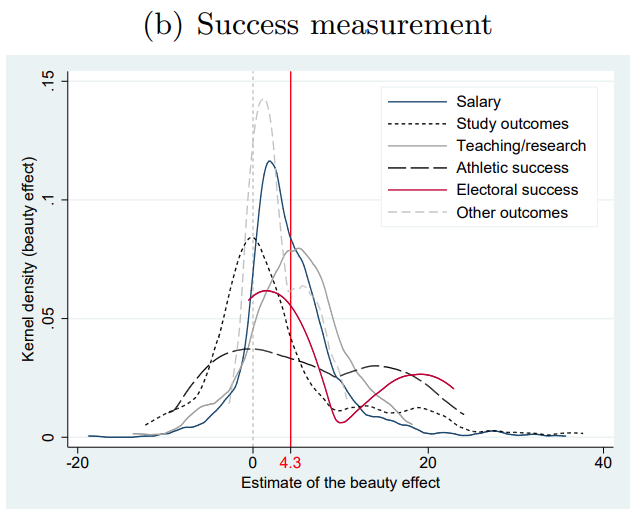
Method doesn't matter

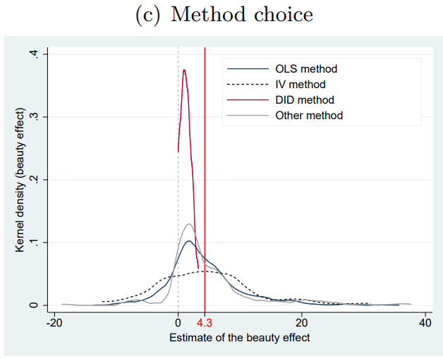
Ability control matters

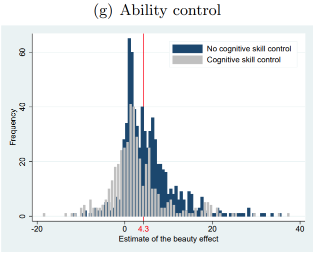
Occupation matters

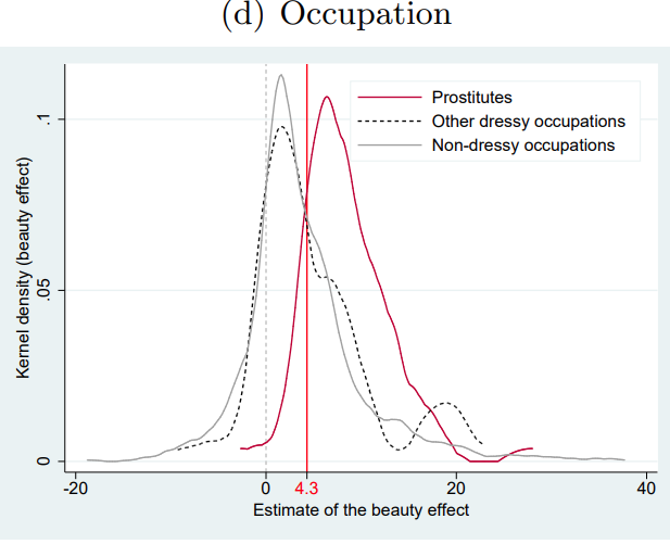
Sex workers stand apart

Option 1: subsamples

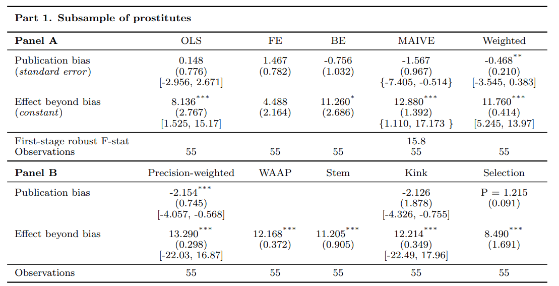
Option 1: subsamples

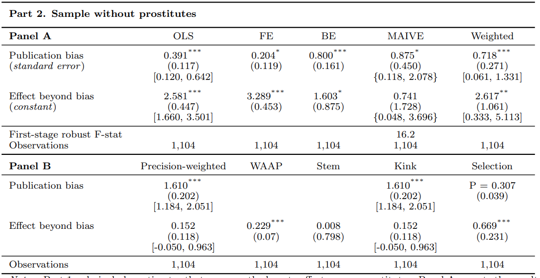
Option 1: subsamples

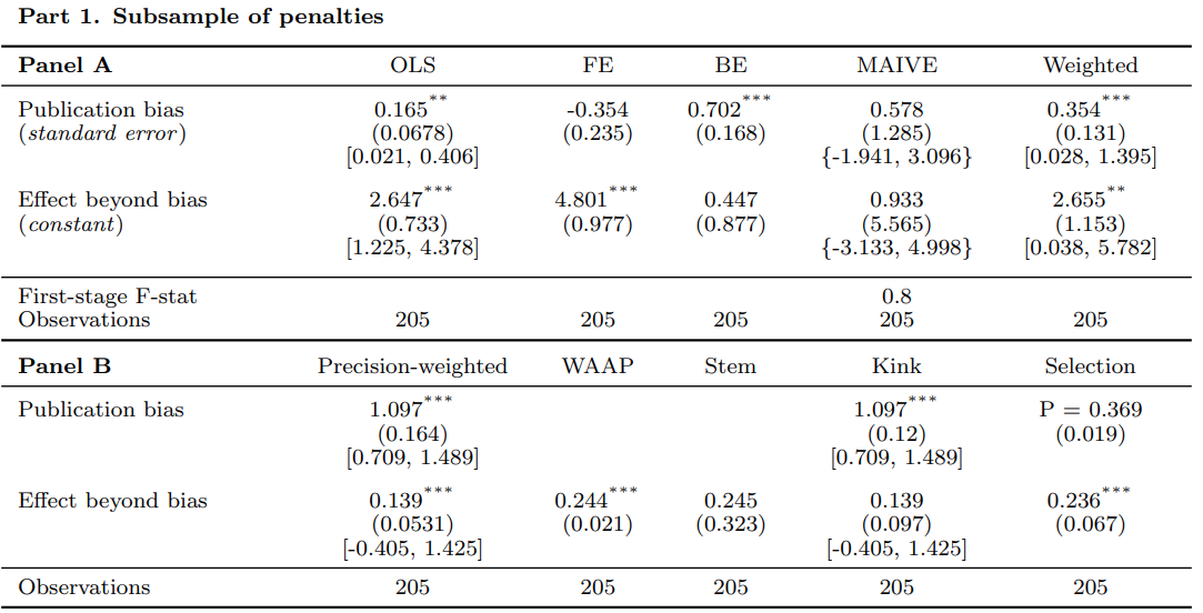
Option 1: subsamples

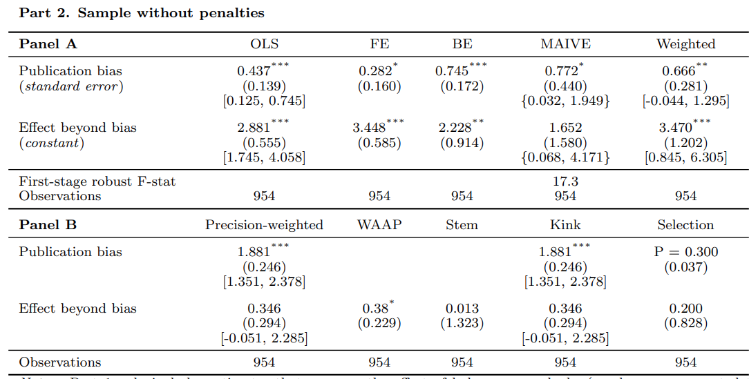
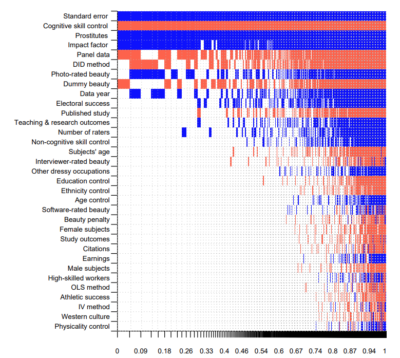
Option 2: Bayesian model averaging

• We want to regress estimates of the beauty effect on variables reflecting heterogeneity
• But too many variables; model uncertainty
• Solution: run regressions with different combinations of the variables
• Give more weight to those that fit the data well and are parsimonious

Option 2: Bayesian model averaging

• Model averaging can be frequentist but computationally difficult
• Intuition: run different combinations and weight by adjusted R^2 or information criteria
• In the Bayesian setting we can use the MCMC algorithm
• G-prior: all coefficients are zero. Weight? UIP = the prior has the same weight as one observation
• Model prior: uniform = all models have the same weight
• Dilution prior: models with collinearity get less weight

Hands on

Open R

Model inclusion in BMA

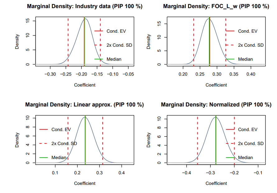
Posterior densities

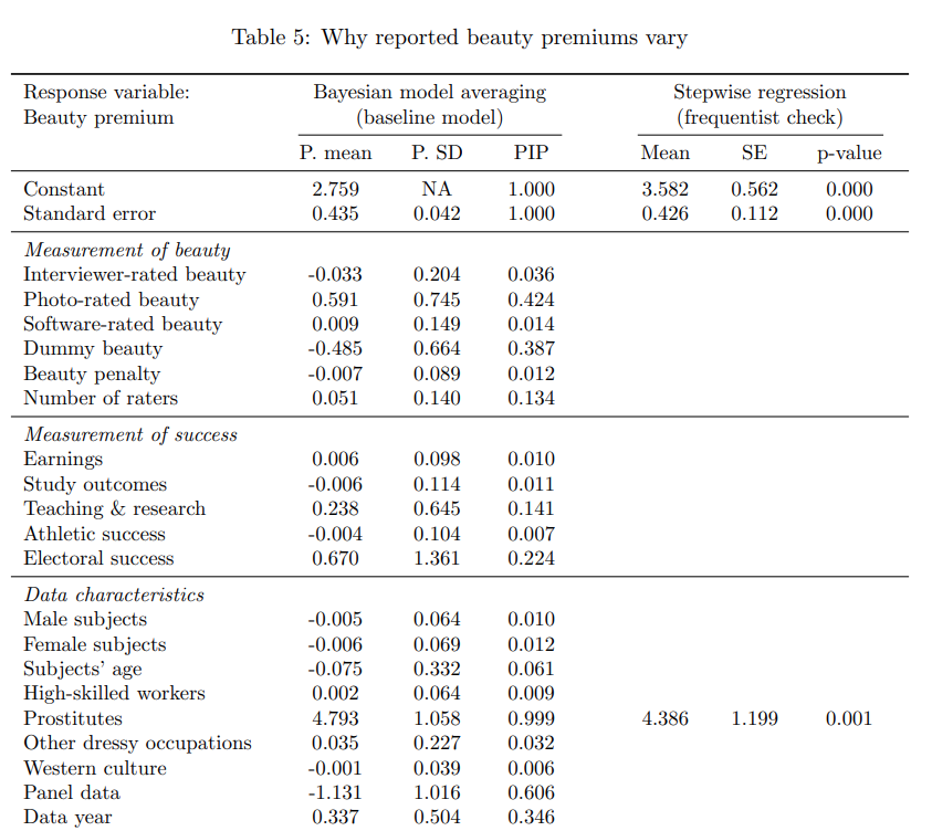
Regression results

Best practice (implied estimate)

• From BMA results we know how estimates depend on study design
• Some study designs are better: identification, data, generally quality
• Select best practice based on the literature (quasi-experimental studies, etc.)
• Compute fitted values and confidence intervals (lincom command in Stata)

Hands on

Open Stata

Best practice (class size effect)

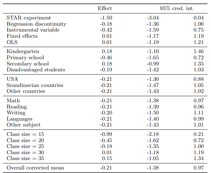
Takeaways

Summary: How to do a modern meta-analysis

1. Search for primary studies using Google Scholar, snowballing, AI agent
2. Use comparable estimates (elasticities, mean differences, correlations)
3. Code standard errors, sample sizes, main differences in data and methods
4. Winsorize estimates and standard errors at the 1% level
5. Correct for publication bias and p-hacking (MAIVE; if weak instrument → RTMA)
6. Examine heterogeneity using BMA with the dilution prior
7. Report implied effects for different contexts

Thank you for inviting me

Prepared for the University of Osaka. Published at meta-analysis.cz/teaching under CC BY 4.0.